
12.2 Mass Transport in Groundwater
In this section, we use the term “mass” to mean anything in the water that isn’t water. Mass occurs in water as dissolved ions, molecules, colloidal particles, or other suspended particles. Mass transport refers to the movement of these dissolved species and particles in groundwater systems.
If we could measure the velocity of groundwater flow at every point in the subsurface and, if we had the computational power to calculate the movement of mass by advection and molecular diffusion at that level of detail, then we could track the movement of mass and predict how its movement would proceed if the groundwater flow field were to change in response to stresses such as recharge events and variable well pumping rates. Given that we cannot fully capture the velocity field in measurements, the hydrogeologic profession has resorted to using a ‘fudge factor6’ that is commonly known as dispersion to represent the complex velocity field that we are not able to measure. Dispersion represents molecular diffusion enhanced by a dispersivity term that accounts for all the spatial and temporal variations of the subsurface velocities that we are not are able to measure and simulate. This difficulty in measuring the details of the velocity field is not unique to groundwater. Another example is our inability to measure the details of velocity in the atmosphere, although in the atmosphere is it easier to see or at least measure the migration of mass. The problem with measuring the details of velocity in a moving fluid is more readily observed in the atmosphere by, for example, watching the discharge of smoke from a variety of sources, particularly on a windy day.
Thus, instead of using the variable velocity field and molecular diffusion to describe and predict mass movement, we use an average velocity and then include a dispersion component to account for the velocity variations that disperse mass. In most situations diffusion is a trivial contributor to mass movement so the diffusion process is ‘lumped’ into the dispersion term that represents the variable velocity field that we are not able to measure. Ultimately, for the purpose of using mathematics to describe and predict mass transport in groundwater, two processes are used: advection and dispersion.
Advection
Groundwater flowing through a porous medium carries dissolved species and particles along with it by a process called advection. Figure 90a shows purely advective mass transport from a continuous source of contamination. The cross hatched area signifies the source zone of the contamination that is maintained at a constant value of concentration—for example, a settling pond, a leaking underground storage tank—and the gray area represents the contamination in the groundwater at the time (t) required for the contaminant to move 50 meters. Figure 90 displays conditions at 500 days for a groundwater velocity of 0.1 m/d. The concentration of contamination is constant throughout the gray area.
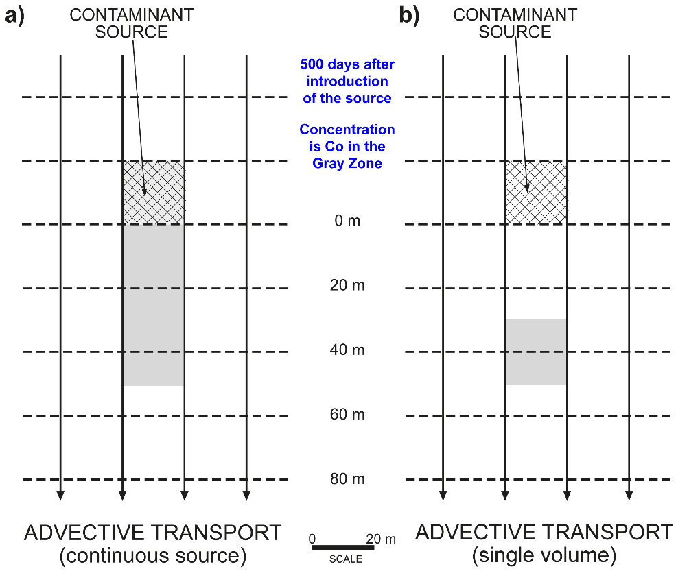
Figure 90 ‑ Position of a plume (light gray) by advective transport 500 days after the source is introduced given a groundwater velocity of 0.1 m/d. a) For a continuous source that is 20 m by 20 m and is maintained at a concentration of Co starting at time zero. b) For a single volume containing contaminant at a concentration of Co that occupies a 20 m by 20 m block of the aquifer at time zero.
Figure 90b shows purely advective mass transport from a single volume of contamination, also called a pulse or a slug, released from a rectangular area at a point in time. The cross hatched area represents the location of the contamination release—for example, a spill from an oil tanker—and the gray area represents the contamination in the groundwater at the time (t) required for the contaminant to move 50 meters. The concentration of the contaminant in the gray area is the same as it was at the initial release.
Advective transport is a function of the velocity of the groundwater. If we assume that advective transport is the only process moving the contaminant, and we know the hydraulic conductivity and effective porosity of our aquifer, we can calculate a travel time, which is the time necessary for the contaminant to move a specific distance ([latex]L[/latex]), using the following procedure.
- Calculate the average linear velocity using Darcy’s law and the effective porosity, as shown in Equation (93):
| [latex]v_{avg} = - \frac{K}{\varphi_{eff}}\frac{\partial h}{\partial x}[/latex] | (93) |
|---|
where (parameter dimensions are dark green font with mass as M, length as L, time as T):
| [latex]v_{avg}[/latex] | [latex]=[/latex] | average linear velocity (LT-1) |
|---|---|---|
| [latex]K[/latex] | [latex]=[/latex] | hydraulic conductivity (LT-1) |
| [latex]\varphi_{eff}[/latex] | [latex]=[/latex] | effective porosity (:) |
| [latex]\partial h/\partial x[/latex] | [latex]=[/latex] | hydraulic gradient (:) |
- Divide the distance ([latex]L[/latex]) by the average linear velocity to get travel time.
Thought Question 11: This assumes that the mass itself does not affect or influence the pattern of flow. Is there a possibility that the contaminant itself may affect flow? (Hint: review Section 3.3.3).
Breakthrough Curves
A good way of visualizing and understanding mass transport processes is using breakthrough curves. Breakthrough curves are graphs that show the either the spatial distribution of the contaminant at a point in time after release or the temporal distribution of the contaminant at one location from the point of release. Breakthrough curves for the situations in Figure 90a and Figure 90b are given in Figure 91 and Figure 92, respectively.
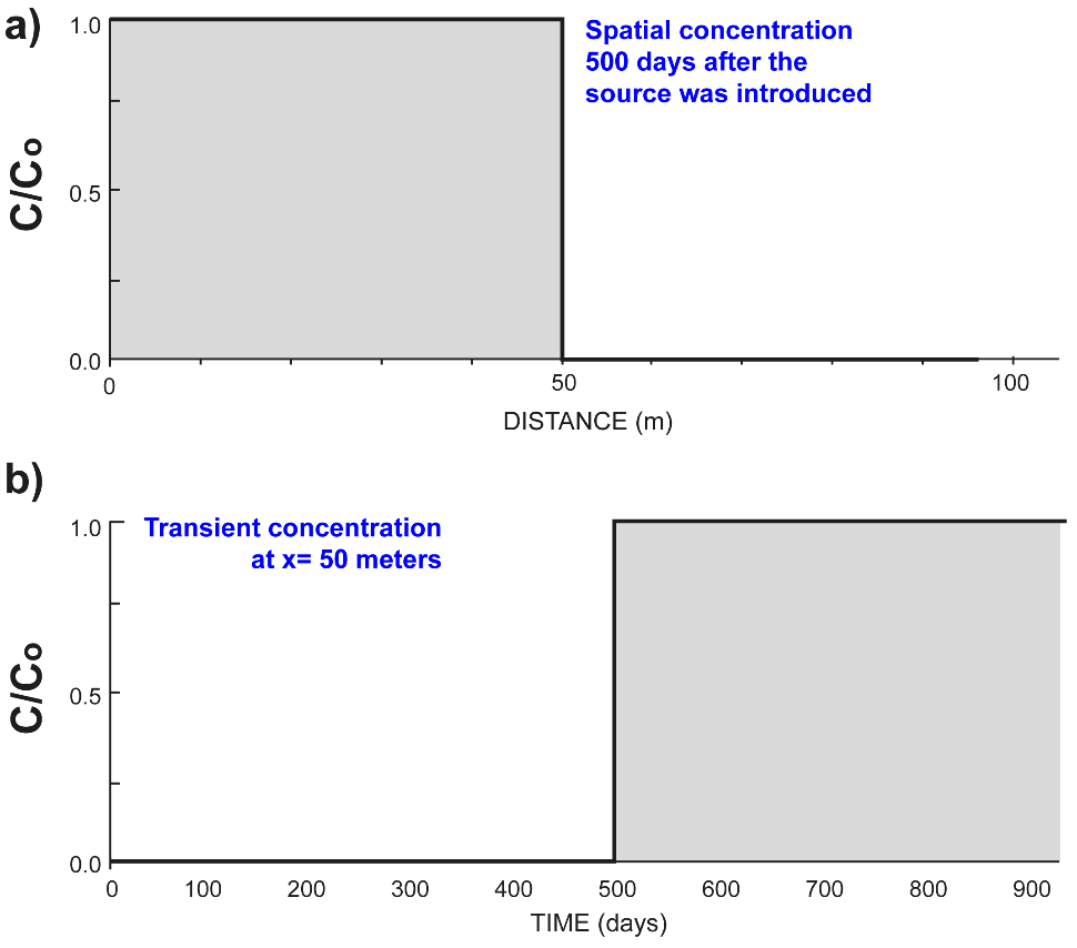
Figure 91 ‑ Concentration, C, relative to initial concentration, Co, for purely advective transport at a groundwater velocity of 0.1 m/d from a continuous source as shown in Figure 90a. a) C/Co as a function of distance from the source 500 days after the source is introduced. b) C/Co at a distance 50 meters from the source as a function of time since the source began releasing contaminants. C/Co changes from zero to one at 500 days, then remains at one until the continuous source is terminated.
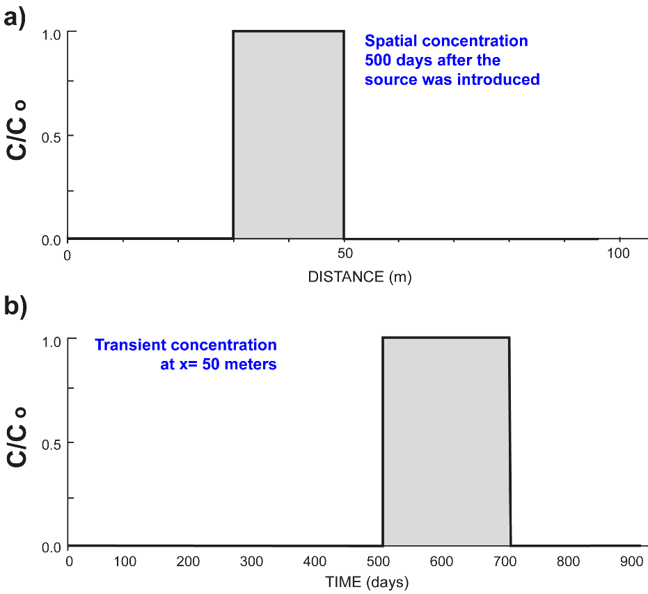
Figure 92 ‑ Concentration, C, relative to initial concentration, Co, for purely advective transport at a groundwater velocity of 0.1 m/d from a single volume source as shown in Figure 90b. a) C/Co as a function of distance from the source 500 days after the source is introduced , and b) C/Co at a distance 50 meters from the source as a function of time since the source was released. C/Co, changes from zero to one at 500 days after the source is introduced, then remains at one until the tail end of the 20-meter-long volume of contaminants moves beyond 50 meters, which occurs 200 days later at 700 days.
The vertical axis on the breakthrough curves represents the concentration of the contaminant ([latex]C[/latex]) divided by the original concentration ([latex]C_{o}[/latex]). This quantity represents the fraction of contamination in the water; where [latex]C[/latex] is the concentration in the water at a given location and time, [latex]C_{o}[/latex] is the source concentration, and [latex]C/C_{o}[/latex] is their ratio. Where [latex]\frac{C}{C_{o}} = 1[/latex], the contamination is equal to the source contamination. The ratio, [latex]C/C_{o}[/latex], can be multiplied by the source concentration to determine the concertation at that location and time.
Concentration of contamination is usually expressed as a mass per volume of water (e.g., mg/L) or as a dimensionless mass per mass (e.g., parts per million). Using [latex]C/C_{o}[/latex] is a dimensionless way of expressing the concentration as a fraction or percentage of the original total concentration, and we use it here to illustrate the basic concepts of contaminant transport.
Dispersion
In groundwater systems, advection is usually the process responsible for moving the largest quantity of mass. However, as the contaminant moves through the subsurface, several processes act on it and cause contamination to spread, resulting in variation of concentration throughout the contaminated area. This spreading of contaminants in the subsurface is called dispersion, or sometimes hydrodynamic dispersion. Dispersion parallel to the flow direction is called longitudinal dispersion, while dispersion perpendicular to the flow direction is called transverse dispersion. Longitudinal dispersion spreads out the contaminant in the direction of flow, while transverse dispersion spreads it out laterally—perpendicular to the direction of flow—as the contaminant moves with flowing groundwater. Although dispersion acts in all directions it is often simplified into longitudinal, transverse lateral, and transverse vertical components.
Dispersion is caused by two processes. The first is molecular diffusion, which is the net movement of dissolved solutes under the influence of a concentration gradient—that is, from areas of high concentration to areas of low concentration. This process is driven by the random motions of the dissolved ions and is a function of the temperature of the water; that is, higher temperatures [latex]=[/latex] more energetic and lively ions [latex]=[/latex] more diffusion. It is possible to measure a diffusion coefficient—a parameter that relates concentration to the rate of diffusion—for various chemicals under laboratory conditions.
All spreading beyond that caused by diffusion is by a second process called hydrodynamic (or mechanical) dispersion. Hydrodynamic dispersion is caused by variations in groundwater velocity (i.e., local variations in magnitude and direction of flow) along the tortuous paths taken by groundwater as it moves through pore spaces and regions of different hydraulic conductivity from point to point in a groundwater system—this is also discussed in sub‑section 3.3.7 Fluid Velocity. Dispersion occurs at the pore scale and at larger scales. In nearly every situation, spreading is greater in the direction of flow, which is described as longitudinal spreading, while spreading in other directions is called transverse spreading. The variations become more complex as transient stresses on the groundwater flow field such as recharge events and well pumping, or other human impacts, shift flow paths over time. Another example of human impact on groundwater flow fields is the presence of open well bores where groundwater moves vertically to enter flow in different depth zones.
Again, as mentioned in Section 12.2 and repeated here for emphasis, it is not possible to measure all the parameters that control velocity variations in a groundwater system, and even if we could measure them, our computers would not be able to simulate those variations. Some advances have been made in more rigorously measuring the subsurface and in modeling transport in groundwater systems using alternative methods such as fractional calculus, and perhaps someday the mathematical calculation of mass transport in groundwater will be a trivial task. However, until that time, for practical reasons, we use hydrodynamic dispersion as a ‘fudge factor’ to account for the unquantified but significant phenomena of spreading mass in a groundwater flow system. Extremely simplified portrayals of the influence of dispersion on contaminant migration is shown in Figure 93.
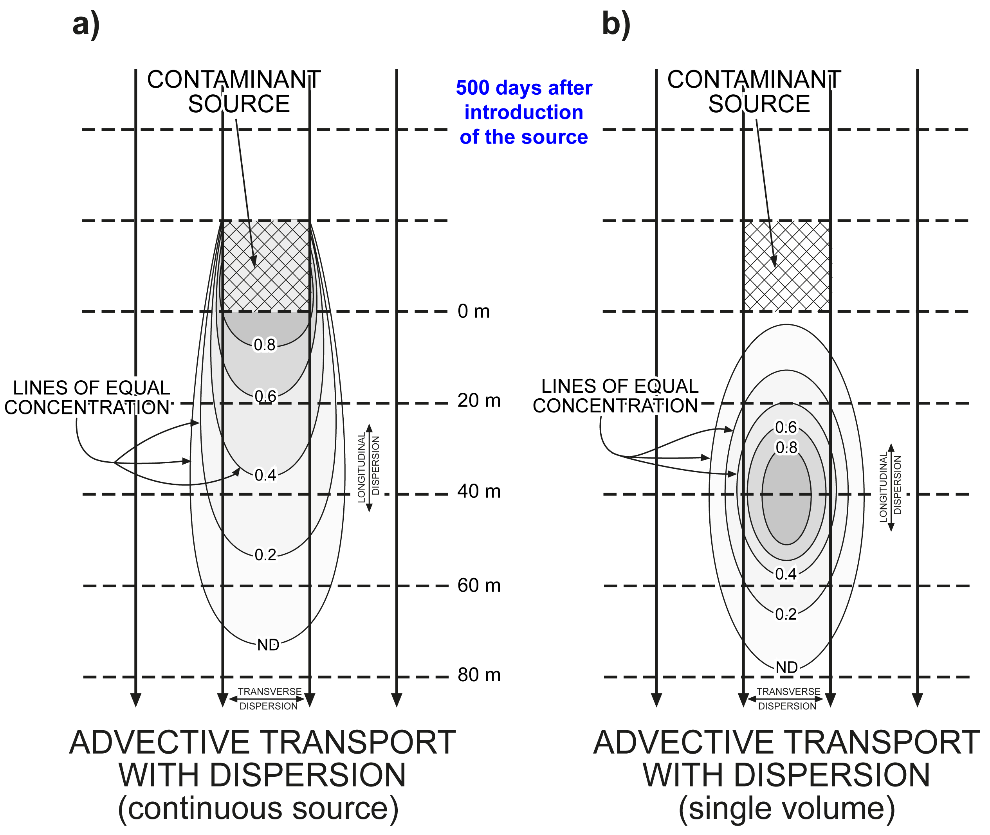
Figure 93 ‑ Advective transport at groundwater velocity of 0.1 m/d with dispersion, showing concentrations relative to initial concentration in the groundwater 500 days after the release of contaminants for the case of a) a continuous source and b) a single volume pulse.
Figure 93a and Figure 93b show the effects of dispersion on contaminant transport from a continuous source and from a single volume pulse of contamination. These figures show the same situation as Figure 90 with the additional process of dispersion. Figure 93a shows advective mass transport with dispersion from a continuous point source of contamination. The cross hatched area signifies the source of the contamination—for example, a settling pond, a leaking under‑ground storage tank—and the lines of equal concentration represent the fraction of the initial contaminant concentration at some time (t) after the release of contamination.
Figure 93b shows advective mass transport with dispersion from a single volume of contamination released from a rectangular source at a specific point in time. The cross hatched area represents the original location of the contamination release—for example, a spill from an oil tanker—and the lines of equal concentration represent the fraction of the initial contaminant concentration at time[latex]\ (t)[/latex] after the release of contamination.
The breakthrough curves for Figure 93a and Figure 93b are shown in Figure 94 and Figure 95, respectively.
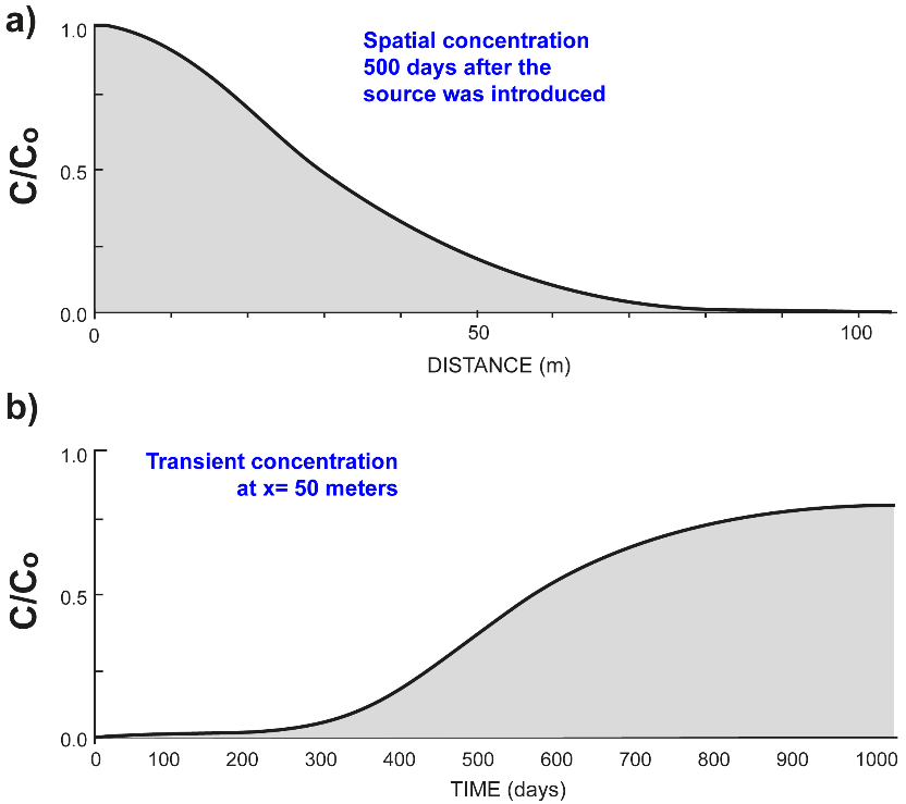
Figure 94 ‑ Concentration, C, relative to initial concentration, Co for advective transport at a groundwater velocity of 0.1 m/d with dispersion from a continuous source as shown in Figure 93a. a) C/Co as a function of distance from the source 500 days after the source is introduced. C/Co never quite reaches a value of one and approaches 1 later than that shown in Figure 91 because dispersion spreads out the contaminants in the aquifer. b) C/Co at a distance 50 meters from the source as a function of time since the source began releasing contaminants. C/Co begins to exceed a value of zero early as a few molecules of contaminants move rapidly ahead, then and rises slowly, never reaching one because the contaminants spread laterally.
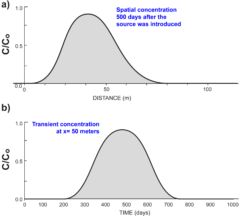
Figure 95 ‑ Concentration, C, relative to initial concentration, Co, for advective transport at a groundwater velocity of 0.1 m/d with dispersion from a single volume source as shown in Figure 93b. a) C/Co as a function of distance from the source 500 days after the source is introduced. b) C/Co at a distance 50 meters from the source as a function of time since the source was released. C/Co rises slowly earlier than for the purely advective transport because some contaminants move rapidly out ahead of the rest. C/Co never reaches one because the contaminants spread laterally.
Thought Question 12: How does the dispersivity affect the shape of the breakthrough curves—that is, what would a curve with a large dispersivity look like versus one with a small dispersivity?
6 A “fudge factor” is a variable included in an equation or calculation to account for some unquantified but significant phenomenon or to ensure a desired result.