
2.2 Fluid Energy
In simple, everyday terms, we think of hydraulic head as an elevation. More specifically, hydraulic head is the elevation of water in a manometer in a pressurized water pipe (Figure 6) or in a piezometer (Figure 7).
- A manometer is a vertical tube in a pressurized water pipe and is used to measure fluid pressure in the pipe.
- A piezometer is a vertical tube with an open or slotted interval—usually called the screened interval or the well screen—inserted into the ground and used to measure hydraulic head in an aquifer; it is basically a well that was constructed for the sole purpose of measuring groundwater levels.
The water level in a piezometer is a manifestation of the total fluid energy in a groundwater system so measuring a water elevation in a well is a measurement of the energy present in the fluid at a certain point in a groundwater system—that is, the interval of the piezometer that is open to the aquifer (Figure 7).
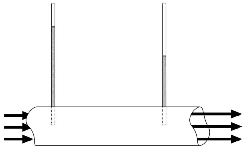
Figure 6 ‑ Pipe of flowing water with manometers showing the loss of head along the flow path.
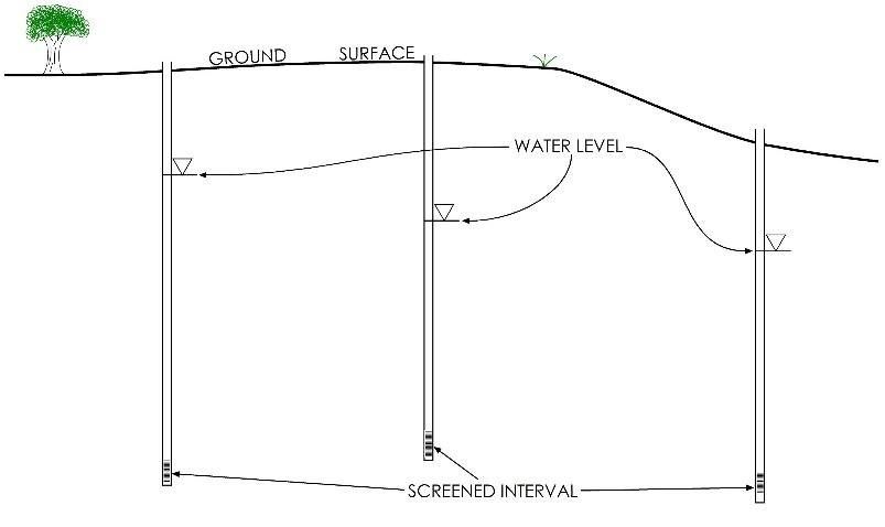
Figure 7 – Cross‑section of aquifer showing hydraulic heads in three piezometers. The line with an inverted triangle represents the depth to which water rises within each piezometer.
The fluid energy in an aquifer varies throughout the aquifer and is different from one point to the next. This results in different water levels in piezometers located at different points throughout the aquifer, and these variations in water level represent variations in fluid energy that in turn drive the movement of water throughout the aquifer. As a result, an aquifer is a dynamic system of flowing water.
What do we mean by Energy?
Everything in the universe has some amount of energy associated with it, and that energy is present in various forms. Variations in energy are what drive all natural processes. The key to understanding physical processes is in understanding the distribution of energy in a system. We differentiate between potential energy and kinetic energy.
Potential energy is energy stored in a piece of matter or at a point in a system. It is generally associated with position within a system (measured as an elevation or distance above a datum) or with the thermodynamics of the system (measured as pressure, temperature, or chemical potential).
Kinetic energy is energy associated with motion and is generally measured as a velocity.
At every point in an aquifer, the fluid possesses some total amount of energy that is the sum of all the potential and kinetic energies in the fluid. The fluid energy at a point in an aquifer manifests itself as the water level in a piezometer. We can also say that the water level, or hydraulic head, represents the total energy in the aquifer at a given point, and we can use the various energy components of the hydraulic head—elevation, pressure, velocity, and so on—to understand the driving forces behind fluid motion in the subsurface.
The Bernoulli Equation
Fluid energies—and, subsequently, water levels—vary from one point in an aquifer to the next. Let us consider the first and second laws of thermodynamics. The first law of thermodynamics states that energy is conserved in any system; that is, it cannot be created or destroyed, and any changes in energy must be accounted for in any system as shown by Equation (3).
| energy added− energy subtracted = change in total energy | (3) |
|---|
This is the same as the conservation of mass, Equation (1), but stated for energy in a system. We could also express the first law in terms of the difference in energy at two points in a dynamic system as described by Equation (4).
| [latex]{total\ energy}_{(at\ point\ 1)} + {energy\ added\ or\ lost}_{(betwen\ point\ 1\ and\ 2)} = {total\ energy}_{(at\ point\ 2)}[/latex] | (4) |
|---|
The second law of thermodynamics states that isolated systems tend to move towards increasing entropy. In a dynamic system like an aquifer, water moves from a point of higher energy (i.e., lower entropy) to a point of lower energy (higher entropy); in other words, groundwater spontaneously moves in the direction of decreasing hydraulic head. It is important to recognize that groundwater does NOT (necessarily) flow downhill relative to the land surface—it flows in the direction of decreasing hydraulic head.
The Bernoulli equation shown in Equation (5) describes the total energy of a fluid at all positions along a flow path in a closed system and is basically an expression of the first and second laws of thermodynamics.
| [latex]z_{1} + \frac{p_{1}}{\rho_{w}g} + \frac{v_{1}^{2}}{2g} + H_{a} = z_{2} + \frac{p_{2}}{\rho_{w}g} + \frac{v_{2}^{2}}{2g} + H_{L} + H_{E}[/latex] | (5) |
|---|
where (parameter dimensions are dark green font with mass as M, length as L, time as T):
| [latex]z[/latex] | [latex]=[/latex] | elevation (L) |
|---|---|---|
| [latex]p[/latex] | [latex]=[/latex] | pressure (ML-1T-2) |
| [latex]\rho_{w}[/latex] | [latex]=[/latex] | fluid density (ML-3) |
| [latex]g[/latex] | [latex]=[/latex] | gravitational acceleration (LT-2) |
| [latex]v[/latex] | [latex]=[/latex] | velocity (LT-1) |
| [latex]H_{a}[/latex] | [latex]=[/latex] | heat energy added (L) |
| [latex]H_{L}[/latex] | [latex]=[/latex] | mechanical energy lost (L) |
| [latex]H_{E}[/latex] | [latex]=[/latex] | heat energy extracted (L) |
| subscripts | [latex]=[/latex] | represent two different positions along the flow path |
If we assume that no heat energy is added to or subtracted from the system, and that the only change is the loss of mechanical energy from one point to the next, we can rewrite the equation as Equation (6).
| [latex]z_{1} + \frac{p_{1}}{\rho_{w}g} + \frac{v_{1}^{2}}{2g} + I_{1} = z_{2} + \frac{p_{2}}{\rho_{w}g} + \frac{v_{2}^{2}}{2g} + I_{2}[/latex] | (6) |
|---|
Where I is the internal energy at each point (i.e., the remainder of the potential energy not described by the other terms) and [latex]I_{2}\ - \ I_{1}[/latex] is equal to [latex]H_{L}[/latex] in Equation (5).
We can understand this equation by considering each individual term in the equation as representing a specific component of energy—that is:
- elevation,
- pressure,
- kinetic (velocity), and
- other internal energies (thermal, chemical).
The equation therefore describes the change in energy from one point along a flow path to the next. The interesting thing about it to us as hydrogeologists is that, since it expresses all the components of energy in the same units (i.e., length), we can use it to compare the relative magnitude of the individual components. When we do that, we see that for most groundwater situations the flow velocity is slow so we can ignore the internal and the kinetic (velocity) components because they are so much smaller than the elevation and pressure components. We can also use the equation to mathematically “convert” one form of energy to another—for example, we can calculate how much a certain change in elevation will result in a change in pressure.
Hydraulic Head and Hydraulic Potential
If we go with the assumption that we can ignore velocity and internal energy components when dealing with groundwater, we can drop all that out of the equation and express the fluid energy as the sum of the elevation and pressure components. That sum is what we call hydraulic head; in physical terms, it is the fluid energy per unit weight, and in mathematical terms, it is described by Equation (7).
| [latex]h = z + \frac{p}{\rho_{w}g}[/latex] | (7) |
|---|
where (parameter dimensions are dark green font with mass as M, length as L, time as T):
| [latex]h[/latex] | [latex]=[/latex] | hydraulic head (L) |
|---|---|---|
| [latex]z[/latex] | [latex]=[/latex] | elevation (L) |
| [latex]p[/latex] | [latex]=[/latex] | pressure (ML-1T-2) |
| [latex]\rho_{w}[/latex] | [latex]=[/latex] | fluid density (ML-3) |
| [latex]g[/latex] | [latex]=[/latex] | gravitational acceleration (LT-2) |
If we multiply both sides of the equation by gravitational acceleration ([latex]g[/latex]), we get a quantity called hydraulic potential ([latex]\Phi[/latex]; i.e., the Greek letter phi), which is the fluid energy per unit mass, as shown in Equation (8) and Equation (9).
| [latex]\Phi = gz + \frac{p}{\rho_{w}}[/latex] | (8) |
|---|
such that
| [latex]\Phi = gh[/latex] | (9) |
|---|
The hydraulic potential is simply a way of expressing the same fluid energy so that it is independent of gravity (in case you would want to compare a typical aquifer on Earth with, say, the liquid methane aquifers on Titan). We do not deal with hydraulic potential any further in this book; hydraulic head is sufficient for the problems that are addressed in this book.
Physical Description of the Components of Head
From Equation (7), we can see that hydraulic head is the sum of the elevation component (or elevation head) and the pressure component (or pressure head). The physical meaning of pressure head and elevation head are defined and described in Figure 8. This figure shows an idealized cross‑section of a piezometer with a screened interval at the bottom. Figure 8a shows the depths and elevations measured in the field. Figure 8b shows the pressure, elevation, and total heads relative to a datum. In this case, the datum is mean sea level.
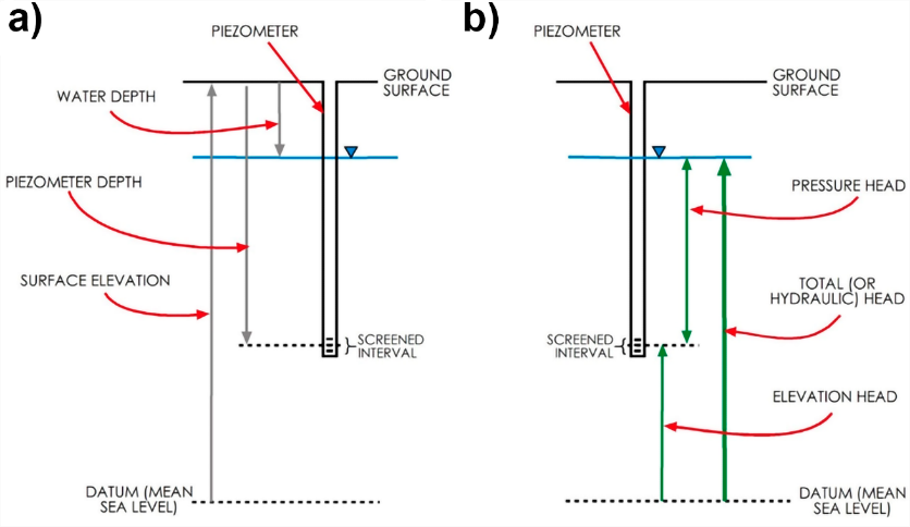
Figure 8 ‑ Hypothetical well showing depths, elevations, and heads.
From Figure 8b, we see that the elevation head is the height of the screened interval above the datum. The datum is arbitrarily chosen—if we wanted, we could choose the middle of the screened interval as the datum, and the elevation head would be zero. However, it is important to realize that hydraulic head is only useful to us when we are looking at multiple wells in the same aquifer, and we need to have a constant datum for all those wells in order to make the comparison meaningful. Sea level is usually chosen, but it is not necessary that we choose that as the datum.
We see from Figure 8b that the pressure head is the length of the column of water in the well above the screened interval. Keep in mind that pressure and pressure head are two different things. The pressure at the screened interval is the force per unit area of the column of fluid above that point, while the pressure head is the pressure divided by the product of the density of the fluid and gravitational acceleration and is manifest as the length of the column of water above the screen. If we know the density of the fluid and the length of the column of water in the well, we can calculate the pressure at the well screen.
Finally, we see that the total head is just the sum of the other two heads or, more generally, the height of the water level in the well above the datum. This brings us back to the concept that the water level in a well is a direct measure of the fluid energy (Exercise 1⮧).
Distribution of Head (i.e., fluid energy) in a 3‑D Aquifer
There are three types of mathematical quantities:
- scalar quantities have magnitude only (e.g., temperature);
- vector quantities have both magnitude and direction (e.g., velocity); and,
- tensor quantities have magnitude that varies with respect to direction (e.g., stress).
Head is a scalar quantity; it is measured at a point, and it has a single magnitude that doesn’t vary with respect to direction. Therefore, when we talk about hydraulic head from a theoretical standpoint, we are talking about the fluid energy at an infinitesimal point in an aquifer. An aquifer, however, exists in three dimensions and contains an infinite number of points, and the head within an aquifer varies from point to point.
The trends in that variation are what control the directions and magnitudes of groundwater flow in an aquifer. We call this variation the hydraulic gradient. The hydraulic gradient is defined as the change in hydraulic head over a change in length, and it is directly analogous to other physical gradients—for example, topographic slope, thermal gradients, concentration gradients, and so on.
Since hydraulic heads exist in three dimensions, hydraulic gradients are not necessarily horizontal. In reality, most groundwater flow is generally in a horizontal direction, and it is often a realistic assumption to ignore fluid movement in the vertical direction. However, there are many situations where vertical gradients—and, subsequently, vertical flow—are significant (Exercise 2⮧).
Why Do We Care About This?
The important thing to realize here is that when we install a piezometer in an aquifer and measure a water level in that piezometer, we are measuring the fluid energy at a point (in three dimensions) that is located at the well screen. Figure 9 shows three wells; wells b and c are completed at approximately the same depth, while well a is completed in a much shallower interval. The two deep wells indicate a gradient pointing to the right of the page; however, the water level in the shallow well—located between the other two—is much lower than either of the other two wells. This indicates that there is some sort of vertical gradient in the system. It could also indicate that the wells are completed in different geologic units that are not well connected. This is discussed further in later sections of this book (Exercise 3⮧).
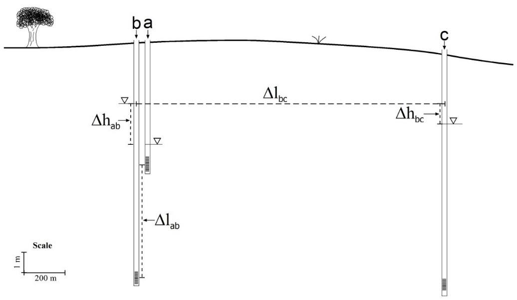
Figure 9 ‑ Cross‑section showing differences in head and their separation that can be used to calculate vertical and horizontal gradients. The large difference in water level of the shallow well (a) which is between wells (b) and (c) suggests there is a vertical gradient in the system, which could reflect that the wells are located in a zone of hydrodynamically-driven upward flow and/or that the wells are completed in different geologic units that are not well connected.
More information about hydraulic head and understanding the relationship between head and groundwater flow can be found in Conceptual and Visual Understanding of Hydraulic Head and Groundwater Flow↗ by Cohen and Cherry (2020), which is available from The Groundwater Project as a free download or can be read online.