
4.4 Groundwater Flow Equations
Darcy’s law is the basic equation that governs the one‑dimensional flow of water in a porous medium. So far, we have treated the gradient term as a simple quantity that can be calculated by dividing the difference in head from one point to the next by the distance between the two points (Figure 17). Also, we have assumed that wells A and B are along a line oriented with steepest head decline for the point of interest.
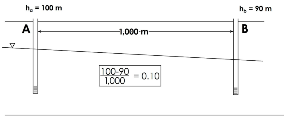
Figure 17 ‑ Cross section showing the overall gradient between two wells.
It is not inappropriate to do this in practice; however, it may not be entirely accurate. The water table could look something like Figure 18. In this case, the gradient is smaller near well A and larger near well B.
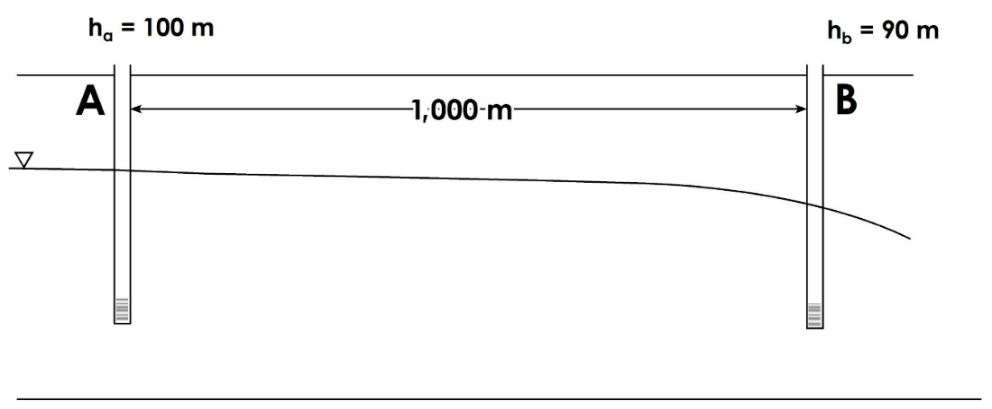
Figure 18 ‑ Cross section showing the water table between two wells.
The hydraulic gradient represents the slope of the water table or potentiometric surface at a point, and that slope varies from one point to the next. In practice, we can occasionally ignore the type of variations shown in Figure 18 and assume that they are not significant. However, it is important to have a basic understanding of the theory and mathematics underlying the hydraulic gradient so that you can decide when it is appropriate to ignore those variations and when it is important to acknowledge them.
Differential Equations
Natural, dynamic, three‑dimensional systems (like aquifers) contain an infinite number of points, and the conditions in those systems vary from point to point. Groundwater flow is driven by a gradient. at each point. A gradient is a slope at a point (i.e., a rise of a line on a graph divided by the run), which is also known as a derivative. Derivatives are the underlying basis of differential equations. So, we use differential equations to describe and understand groundwater systems.
A derivative is the instantaneous change in a parameter with respect to some independent variable. In Darcy’s law, the hydraulic gradient is a derivative. Figure 19 graphically shows the slope of the water table over progressively smaller intervals (Figure 19a through c) with Figure 19d showing the slope at an infinitesimally small distance (i.e., at a point). We use the symbol [latex]\mathbf{\mathrm{\Delta}}[/latex] to indicate a finite amount of change in a parameter; for example, [latex]\mathrm{\Delta}h[/latex] refers to a specific change in head over a given lateral distance ([latex]\mathrm{\Delta}l)[/latex].
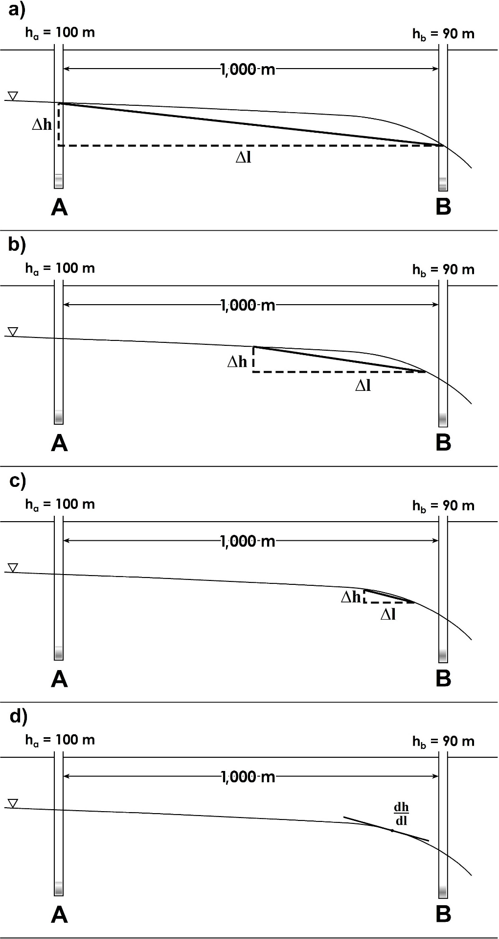
Figure 19 – a), b), c) Illustration of hydraulic gradient as a slope along progressively smaller finite distances ([latex]\mathrm{\Delta}h/\mathrm{\Delta}l[/latex]) and d) as an infinitesimal derivative at a single point ([latex]dh/dl[/latex]).
In a differential equation, we use the symbol d to signify the infinitesimal change in magnitude of a parameter (e.g., head) with respect to some independent variable (e.g., length along the flow path). So, for Darcy’s law, we are looking at the hydraulic gradient at a single point in a single direction (along the length of the flow path), and the derivative dh/dl represents the gradient in that direction at that single point.
Since groundwater flow (i.e., [latex]q[/latex]) is driven by the gradient, q also varies from one point to the next. So, we can think about the change in flow with respect to length as [latex]\frac{dq}{dl}[/latex].
An aquifer, however, exists in three dimensions and contains an infinite number of points, and at each point groundwater is flowing in some direction. Let’s choose a single point in our aquifer and consider how groundwater is flowing at that point (Figure 20). At this point groundwater is flowing in some unique direction. We can represent the flow direction and magnitude with a vector (i.e., an arrow), and define a three‑dimensional coordinate system (the [latex]x,\ y[/latex], and [latex]z[/latex] arrows) to provide a frame of reference. Any vector within a coordinate system can be resolved into component vectors in the principal ([latex]x,\ y[/latex], and [latex]z[/latex]) directions. What this means is that the three component vectors add up to the groundwater flow vector.
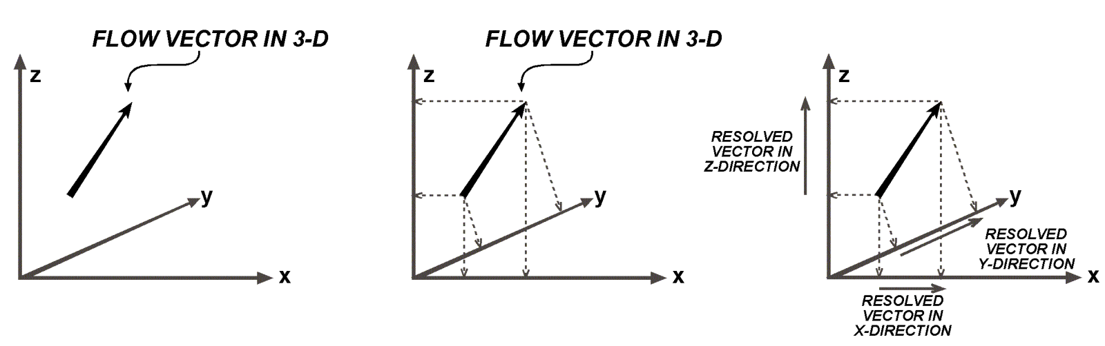
Figure 20 ‑ Vector resolved into component vectors in three dimensions.
Each one of the component vectors represents the flow (i.e., [latex]q[/latex]) in each of the principal directions. There is a [latex]q[/latex] in the x direction ([latex]q_{x}[/latex]), in the y direction ([latex]q_{y}[/latex]), and in the z direction ([latex]q_{z}[/latex]). When we have a derivative that has multiple independent variables (i.e., the three directions), we use a partial differential equation, which uses the symbol [latex]\partial[/latex] instead of [latex]d[/latex] to indicate the change in magnitude of a variable with respect to the independent variable in each direction. We can then express that flow vector using partial differentials as [latex]\left( \frac{{\partial q}_{x}}{\partial x} + \frac{{\partial q}_{y}}{\partial y} + \frac{{\partial q}_{z}}{\partial z} \right).[/latex]
Generally, groundwater flow varies with time and we can equate the flow vector to the change in water stored in the system over an infinitesimally small time (i.e., a derivative of water level, h, with time, t) as expressed by the partial differential equation shown as Equation (34).
| [latex]\frac{{\partial q}_{x}}{\partial x} + \frac{{\partial q}_{y}}{\partial y} + \frac{{\partial q}_{z}}{\partial z} = S_{s}\frac{\partial h}{\partial t}[/latex] | (34) |
|---|
where (parameter dimensions are dark green font with mass as M, length as L, time as T):
| [latex]\mathbf{S}_{\mathbf{s}}[/latex] | = | the specific storage (L-1), which is a coefficient that relates changes in hydraulic head to changes in volume of water stored in a unit volume of aquifer. This term is defined in more detail in Chapter 5. |
|---|
Darcy’s law (expressed as the specific discharge) is shown again here in Equation (35).
| [latex]q = - K\frac{dh}{dl}[/latex] | (35) |
|---|
So, we can substitute it for [latex]q[/latex], to obtain Equation (36).
| [latex]\frac{\partial\left( K_{x}\frac{\partial h}{\partial x} \right)}{\partial x} + \frac{\partial\left( K_{y}\frac{\partial h}{\partial y} \right)}{\partial y} + \frac{\partial\left( K_{z}\frac{\partial h}{\partial z} \right)}{\partial z} = S_{s}\frac{\partial h}{\partial t}[/latex] | (36) |
|---|
This is the primary groundwater flow equation, which describes the flow of groundwater at every point in a flow system. The left side of this equation is called the divergence of flux because it represents the amount of flux entering or leaving a point.
What Does This Mean in Conceptual Terms?
This is just a more complex version of the continuity equation; each term on the left is:
[latex]I - O[/latex] (what goes in minus what goes out)
for each direction (x, y, and z) for a given point in the flow system, and the term on the right is:
[latex]\mathrm{\Delta}Storage[/latex](change in storage)
for that point in the system.
In a 3‑D flow system, there are an infinite number of points, and an infinite number of equations that describe flow through each point. We cannot simply plug a few values into the equation and directly solve it; instead, we must use some indirect method to solve the equation.
How Do We Solve These Equations?
We use one of several methods to solve the partial differential equations that represent natural systems.
Flow nets are a graphical representation of a groundwater flow system that can be used to identify flow paths in an aquifer and estimate hydraulic conductivity. More information on constructing and using flow nets can be found in Graphical Construction of Groundwater Flow Nets↗ by Poeter and Hsieh (2020), which is available from The Groundwater Project as a free download or can be read online.
Analytical equations are solutions of the groundwater flow equation for specific situations, such as a system with a simple geometry. An example of an analytical solution to the 3‑D groundwater equation—i.e., Equation (36)—is the Theis equation, which solves for radial flow to a pumping well with a specific set of assumptions. The Theis equation is discussed in more detail in Section 7.
Numerical solutions involve discretizing a system—that is, reducing the infinite number of points/equations to a finite number and simultaneously solving that set of equations. For numerical solutions, each individual equation is generally dependent on the values for the surrounding equations, often in a non-linear manner; therefore, the equations need to be solved using an iterative method that requires a computer and specialized software. These types of solutions, and the software used to develop them, are generally called computer models. Popular software packages used for developing groundwater flow models include MODFLOW and FEFLOW. Computer models are discussed in more detail in Section 10.
A more detailed discussion of the equations governing groundwater flow can be found in the seventh section of Hydrogeologic Properties of Earth Materials and Principles of Groundwater Flow↗ by Woessner and Poeter (2020), which is available from The Groundwater Project as a free download or can be read online. In addition, a good introduction to using MODFLOW can be found in Getting Started with MODFLOW↗ by Winston (2023), which is also available as a free download from The Groundwater Project.