
13.5 Streams
Streams are generally connected hydraulically to the underlying groundwater. When groundwater is discharging into the stream, we call the stream a gaining stream. The amount of water that flows into the stream from the groundwater is called baseflow. If infiltration causes the water table to rise, the hydraulic gradient between the groundwater and the stream stage will increase and the amount of baseflow will also increase. For many streams, baseflow is the source of water to the stream except during storms, when precipitation in the watershed exceeds the infiltration capacity and the depression storage is filled. In this case, runoff (also called overland flow) will occur, and this runoff will flow into the stream. Natural runoff varies widely in its contribution to the total volume of water flowing through a watershed. In arid regions where the streams are losing streams and are not receiving baseflow, natural runoff is a significant contributor to stream flow. In heavily urbanized areas, with a lot of impervious cover—parking lots, roads, buildings—runoff is a much more significant contribution to the surface water system.
Discharge
Discharge is defined as the volume of water moving past a point on a stream in a given period of time. In the simplest terms, stream discharge ([latex]Q[/latex]) is equal to the velocity of the water ([latex]v[/latex]) times the cross‑sectional area of the stream ([latex]A[/latex]), or [latex]Q\ = \ vA[/latex]. The complication is that water in the stream is flowing fastest in the middle of the stream and slowest at the edges and along the bed of the stream. Figure 104a shows a cross section of a stream flowing into (or out of) the page. Figure 104b shows contours indicating the changes in velocity LT‑1) throughout the stream. The line a–a’ shows the velocity profile; with arrows on the left side representing the magnitude of velocity with direction into, or out of the page.
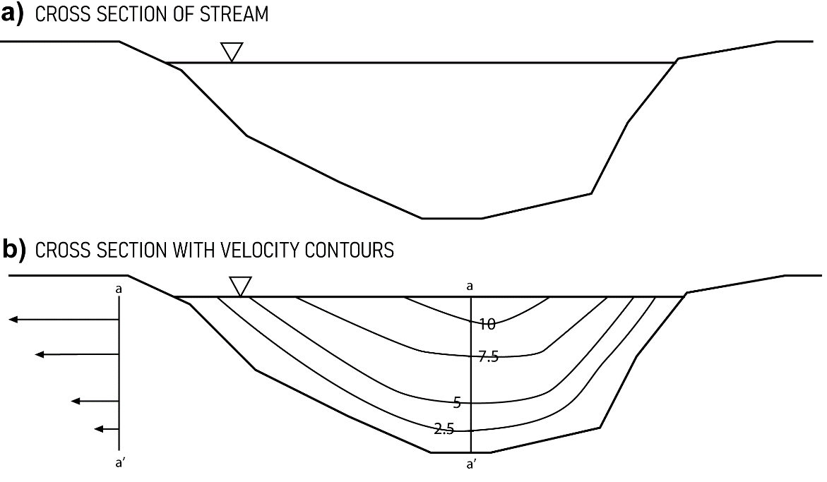
Figure 104 ‑ Cross‑section of stream showing stream profile and velocity contours. The contour values might represent feet per second.
To measure discharge, the average velocity of the water in the stream must be estimated. Stream velocity can be measured at points in the channel using a current meter. Experience has shown that, in water greater than about 2.5 feet (0.76 m) deep, averaging velocity measured at 0.2 and 0.8 of the total depth provides a good average water velocity for the segment. If the stream is less than 2.5 feet (0.76 m) deep, one measurement at 0.6 of total depth is representative of the average velocity (Figure 105). Measurements are made at regular intervals (e.g., 0.5 feet or 0.15 m) across the stream. The velocity is then multiplied by the interval and the depth of the stream in that interval to get a discharge for each vertical strip of the stream. The sum of the individual discharge measurements is the overall discharge of the stream.
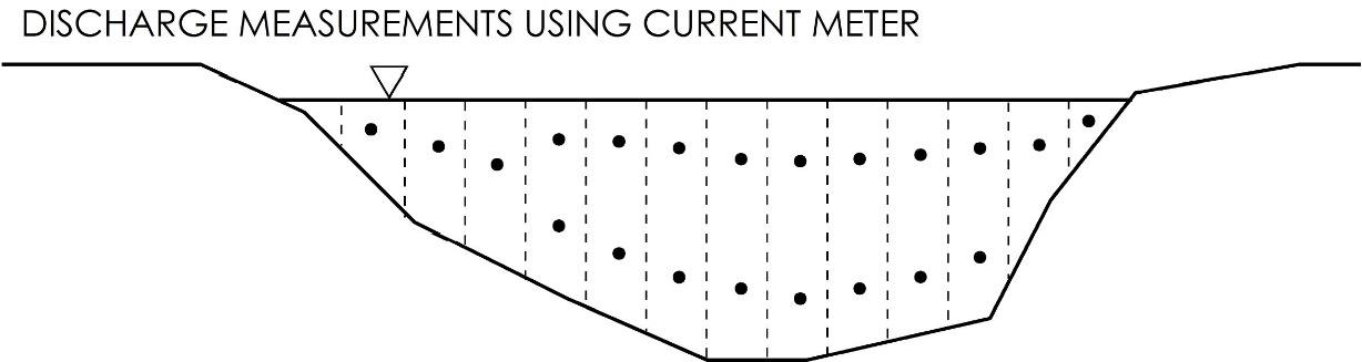
Figure 105 ‑ Cross section of stream showing stream gaging measurement locations.
If a lot of stream gage measurements are made at different times of the year under different flow conditions—that is, low, moderate and high flows—a relationship between stream stage—that is, water surface elevation—and stream discharge can be developed. This is done by repeatedly measuring the stage height each time the discharge is measured, then plotting the values on a graph and connecting them with a curve. This curve is called a stage‑discharge rating curve (Figure 106). The utility of this is that it is much easier to measure stream stage, because once a stage‑discharge curve is developed, only the stage of the stream needs to be measured to estimate discharge.
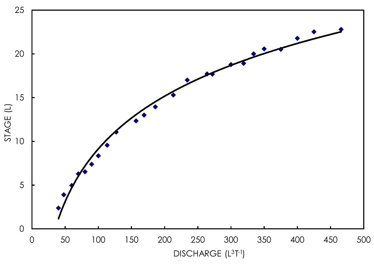
Figure 106 ‑ Stage‑discharge rating curve.
Stage‑discharge rating curves are not linear. This is because the relationship between cross‑sectional area and elevation of the stream water surface is not linear. More specifically, as the river stage increases, the overall area available for water to flow through increases much more dramatically and the discharge increases more rapidly than the stage increases.
Thought Question 13: What might cause the stage‑discharge rating curve for a specific stream to change?
One can also measure stream discharge in small streams using a weir. A weir is a dam with a small opening of a pre‑determined size and geometry that allows water to flow through. The most common weirs are the rectangular weir, the trapezoidal (also called Cipolletti) weir, and the 90° V‑notch weir (Figure 107). The water level just behind the weir blade can easily be measured and used to estimate discharge through the weir opening based on equations that are specific to each weir shape.
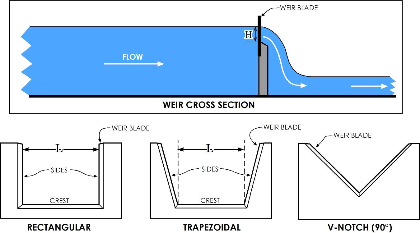
Figure 107 ‑ Different types of weirs.
Equation (103) and Equation (104) are equations for calculating discharge using rectangular and V‑notch weirs respectively.
Rectangular Weir
| [latex]Q\ = \ 3.33(L\ - \ 0.2H)H^{\frac{3}{2}}[/latex] | (103) |
|---|
90° V‑notch Weir
| [latex]Q = 2.5H^{\frac{5}{2}}[/latex] | (104) |
|---|
where these empirical equations need to be used with specific units:
| [latex]Q[/latex] | = | discharge in cubic feet per second (cfs) |
|---|---|---|
| [latex]L[/latex] | = | length of the weir crest in ft |
| [latex]H[/latex] | = | head of the backwater above the weir crest in ft |
These equations are empirically derived, so the coefficients in the equations don’t have any real meaning—they empirically relate water elevation to discharge. The coefficients used here are tied to units of feet, so different coefficients are required if different units are used.
Manning Equation
The average velocity of flow in an open channel can be calculated using the Manning equation as shown in Equation (105) for units of feet and seconds. To use the formula with meters and second, the 1/n is replaced with 1.49/n.
| [latex]v = \frac{1}{n}R^{\frac{2}{3}}S^{\frac{1}{2}}[/latex] | (105) |
|---|
where:
| [latex]v[/latex] | = | velocity (meters per second) |
|---|---|---|
| [latex]R[/latex] | = | hydraulic radius, or the ratio of the cross‑sectional area of flow to the wetted perimeter (meters) |
| [latex]S[/latex] | = | energy gradient (or the slope of the water surface) |
| [latex]n[/latex] | = |
Manning roughness coefficient – values are accessible via internet search (e.g., the engineering toolbox↗) – some examples of its magnitude for streams are provided here.
|
The wetted perimeter refers to the length of the channel that is in contact with the water. The Manning roughness coefficient is an empirically derived number that basically describes how the roughness of the channel creates friction that slows down the water in the channel. As with the weir equations, the Manning equation has empirically derived coefficients that require specific units of feet and seconds.
This equation is a way of determining flow velocity or, indirectly, discharge. It can be used to model streams that don’t exist yet, like a proposed drainage channel for a new housing development. It can also be used to estimate flow in an existing channel under various storm events, provided that the slope and dimensions of the channel are known.
Stream Hydrographs
A stream hydrograph is a graph that represents river discharge at a single point on a river as a function of time. A stream hydrograph shows how discharge in the stream changes with time and, if plotted with precipitation, also shows how discharge responds to storms. A specific hydrograph for a storm event is called a storm hydrograph. Figure 108 shows a typical storm hydrograph.
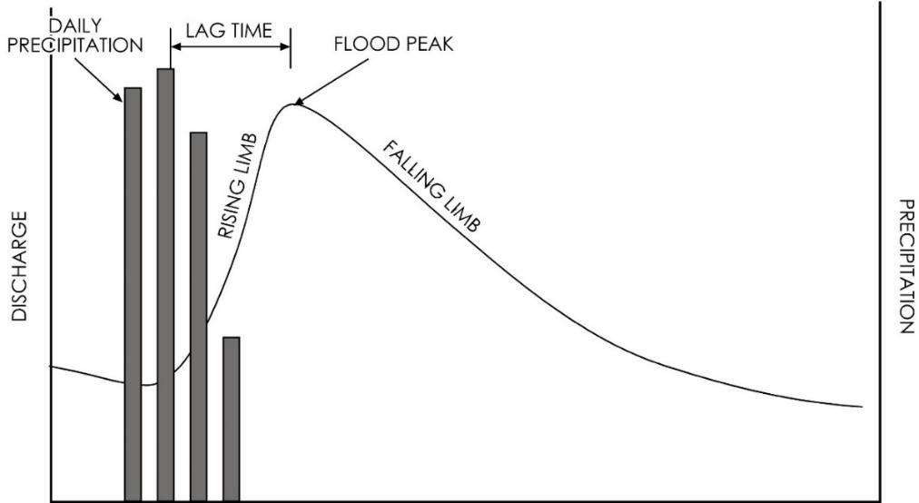
Figure 108 ‑ Hypothetical storm hydrograph showing response to a 4‑day storm event.
The columns represent daily precipitation with the scale on the right axis. The flood peak, or point where flow is highest, occurs at some time after the precipitation peak. This difference in time is called the lag time. The lag occurs because it takes time for water to flow overland or through the subsurface as interflow. The lag time is different for each watershed and is a function of the size and geometry of the watershed as well as the surface conditions and geologic materials in the watershed. The part of the curve that is increasing is the rising limb of the curve; the part that is decreasing as storm water drains out of the watershed is the falling limb.
The hydrograph can be broken up into specific components (Figure 109). The flow in the stream is a combination of baseflow from groundwater and surface runoff from the storm event. The baseflow increases throughout the storm event in response to rising groundwater water levels around the stream. At the point where the runoff from the watershed is exhausted and the stream is fed only by baseflow, the stream is in recession.
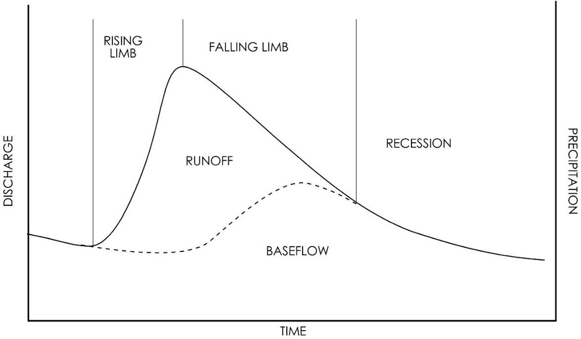
Figure 109 ‑ Storm hydrograph showing the specific parts of the curve.
Thought Question 14: Why are the lag times between the runoff peak and the baseflow peak different?
In the absence of precipitation, the recession part of the hydrograph continues to decrease. Eventually, as the groundwater continues to drain and groundwater levels decline further, the stream stops receiving baseflow from the groundwater, and stream discharge is zero. The shape and slope of the baseflow recession hydrograph is a function of the geometry of the basin as well as the geology and soil characteristics and is unique to each stream.
Thought Question 15: What factors control the shape of the runoff and baseflow parts of the curve?