
10.4 The Method of Finite Differences
The equation applied to each model node is a finite version of the groundwater flow equation, Equation (91). We can re‑state that in the following way. Equation (91) represents the flow at an infinitesimal point, a point with no dimensions. When a finite number of nodes is added to a numerical model, the equation must be transformed so that it accounts for the distance from one node to the next and/or the overall volume of aquifer which is represented by the node. There are several mathematical methods that we can use to do this; the one used in most groundwater models is the method of finite differences.
The exact derivation of the finite difference equations is not presented here, nor a comprehensive overview of the method. Instead, the goal of this section is to provide a very simple and general overview of the procedure. To illustrate the approach in the simplest manner, we can assume that the equations calculate the value of head at each node as an average of the heads at the surrounding nodes. If the aquifer is modeled as heterogeneous, or isotropic, or if the node spacing is variable, it gets a little more complicated than that, but for now we just need to consider that the value at each node is dependent upon the four surrounding nodes.
Each node in a finite difference model grid requires a hydraulic conductivity and a storage parameter—specific yield if unconfined, specific storage if confined. Recharge can be added to each node. This is accomplished mathematically by adding a volume of water per unit time to the node, and the storage parameter controls the resulting head change. Pumping wells can also be added at any node. Pumping wells are the inverse of recharge—that is, a volume of water per unit time is removed. Recharge and wells are specified flux boundaries.
Boundary conditions must be applied to the grid at the edges of the model domain. A no‑flow boundary is treated like an image well problem, with an imaginary node on the opposite side of the boundary with head equal to the active node inside the boundary (Figure 75a). For a constant head boundary, the constant head value is assigned to the node and is not recalculated based on head at surrounding nodes (Figure 75b).
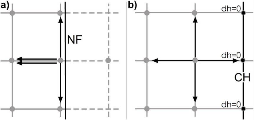
Figure 75 ‑ Implementation of boundary conditions in finite‑difference grids for: a) no‑flow boundary with dashed lines representing the ‘image’ nodes; and b) constant head boundary with black nodes representing locations where head is assigned so it influences calculations as surrounding nodes but is not recalculated during iteration.
Finite difference model grids must follow certain rules. The simplest approach to discretizing a model is to use a consistent row and column spacing throughout the model grid (Figure 76). If there is an area within the center of the overall model domain that requires high resolution—for example, a proposed well field for a new factory—then variable row and column spacing can be applied to the grid (Figure 77). The advantage of this approach is that it uses fewer nodes overall, which makes the model less computationally intensive. A potential disadvantage is that the long rectangular model cells at the edges can create model instability and result in models that do not converge. There are recently developed versions of publicly available groundwater modeling software that utilize unstructured or nested grids, which allow for finer grid resolution within larger grid cells thus avoiding the elongated rectangles at model edges (Figure 78)—for example, MODFLOW‑USG, MODFLOW 6↗. These models allow for more efficient grid spacing with high resolution in some areas and larger grid cells in others.

Figure 76 ‑ Example of a finite difference grid with constant row and column spacing.
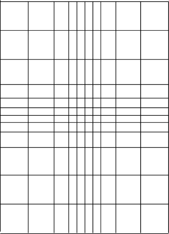
Figure 77 ‑ Example of a finite difference grid with variable grid spacing. This can be applied to a model which has an area in the middle of the model domain that requires high resolution.
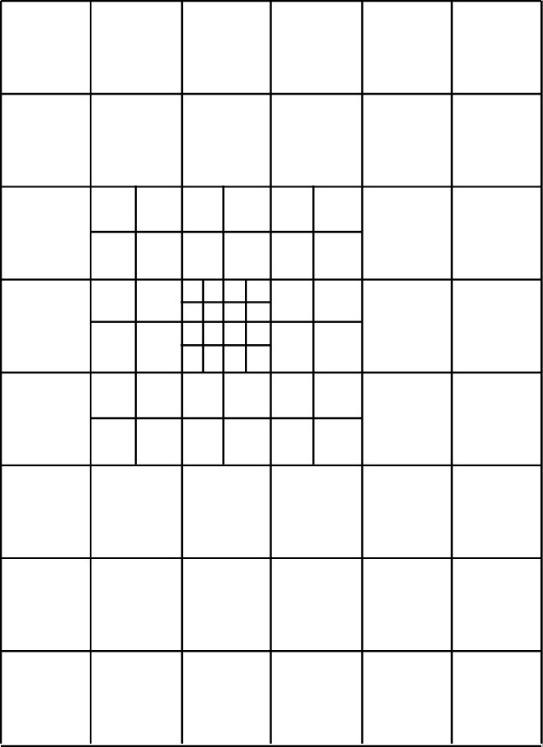
Figure 78 ‑ Example of a finite difference grid with nested grids. This is a more stable and efficient way of simulating high-resolution areas within the model grid as compared to Figure 78.
Figure 79 is an example of an unacceptable finite difference model grid with grid cells that are not rectilinear. There is an alternate model approach called the method of finite elements that allows for variable model elements such as those in Figure 79. The finite element method will not be discussed further in this book.
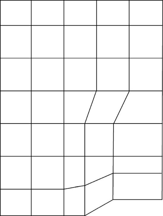
Figure 79 ‑ Example of an unacceptable finite difference grid with non‑rectilinear grid cells.