
6.3 Flow Calculations and Applications of the Flow Equation
The following is a general overview of various ways of quantifying groundwater flow and solving, either directly or indirectly, the groundwater flow equation.
Steady‑State Flow in a Confined Aquifer
In the case of steady‑state flow through a confined aquifer (Figure 28), a change in head does not change the saturated thickness.
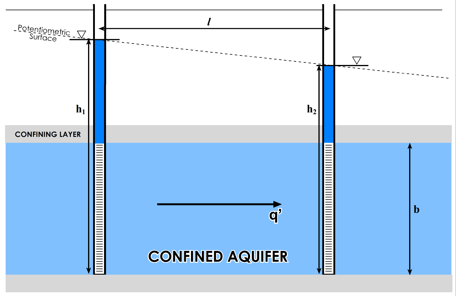
Figure 28 ‑ Steady flow through a confined aquifer of uniform thickness.
We can use a direct variation of Darcy’s law to calculate volumetric flow per unit width of aquifer ([latex]q’[/latex]) as shown in Equation (54).
| [latex]q' = Kb\frac{dh}{dl}[/latex] | (54) |
|---|
where (parameter dimensions are dark green font with mass as M, length as L, time as T):
| [latex]q'[/latex] | = | flow per unit width of aquifer (L2T-1) |
|---|
Given that [latex]Kb\ = \ T[/latex], we could substitute [latex]T[/latex] into the equation for [latex]Kb[/latex].
The head [latex]\left( h' \right)[/latex] at some intermediate distance [latex](x)[/latex] along the flow path can be calculated by Equation (55).
| [latex]h' = h_{1} - \frac{q'}{Kb}x[/latex] | (55) |
|---|
where (parameter dimensions are dark green font with mass as M, length as L, time as T):
| [latex]x[/latex] | = | some distance from [latex]h_{1}[/latex] (L) |
|---|
Steady‑State Flow in an Unconfined Aquifer
Unconfined aquifers are a bit more mathematically complicated because the water table is the upper boundary, and since the water table changes from one point to the next, the saturated thickness ([latex]b[/latex]) changes as well (Figure 29). Since we cannot treat b as a constant, we must use some integral calculus and specific assumptions to develop an equation (based on Darcy’s law) that can be solved directly.
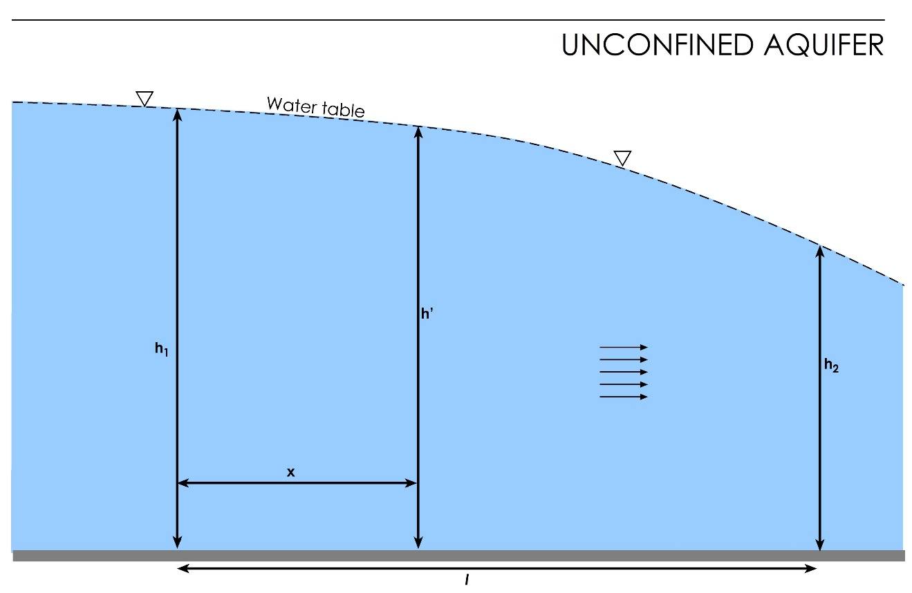
Figure 29 ‑ Steady flow through an unconfined aquifer.
We won’t go through the derivation here, but we discuss the assumptions. This solution was first derived by Dupuit in 1863; hence they are called the Dupuit assumptions. This solution assumes:
- the hydraulic gradient is equal to the slope of the water table, and
- flow is horizontal.
Incorporating these assumptions results in the Dupuit equation that is shown as Equation (56).
| [latex]q' = \frac{1}{2}K\left( \frac{h_{1}^{2} - h_{2}^{2}}{L} \right)[/latex] | (56) |
|---|
Calculating intermediate heads is a problem in an unconfined aquifer because unconfined aquifers usually receive recharge from above the water table (Figure 21). Equations have been derived to calculate heads in an unconfined aquifer with areal recharge. These can be explored using the interactive educational tool called WTR (Water Table Recharge) by visiting https://interactive-education.gw-project.org/wtr/↗ on the Groundwater Project web site (https://gw-project.org/↗).
A more detailed discussion of the equations governing groundwater flow can be found in the seventh section Hydrogeologic Properties of Earth Materials and Principles of Groundwater Flow↗ by Woessner and Poeter (2020) which is available from The Groundwater Project as a free download or can be read online.
Flow Lines and Flow Nets
Another way of solving steady‑state groundwater flow problems is by using flow lines and equipotential lines. A flow line is an imaginary line that traces the path that a particle of groundwater would follow as it flows through an aquifer. Equipotential lines are lines that connect points of equal head in the aquifer. In an isotropic aquifer, the flow lines are perpendicular to the equipotentials and point in the direction of decreasing head. In an anisotropic aquifer, the flow lines will be deflected according to the direction of maximum [latex]K[/latex] (Figure 30).
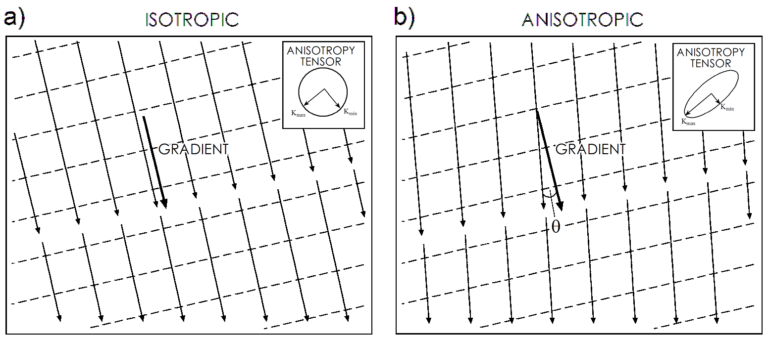
Figure 30 – Equipotentials (dashed) and flow lines (arrows) in isotropic and anisotropic aquifers.
If the degree of anisotropy is known with certainty, there are ways that the amount of deflection (angle θ in the anisotropic diagram, Figure 30b) can be calculated.
A flow net is a graphical representation of the steady‑state groundwater flow equation that depicts equipotentials and flow lines and, if properly drawn, represents a graphical solution to the two‑dimensional Laplace equation—that is, steady‑state flow in a homogeneous and isotropic aquifer. Flow net construction requires the following assumptions.
- The aquifer is homogeneous, isotropic, and fully saturated.
- The aquifer is at steady‑state—heads are not changing with time.
- Flow is laminar and Darcy’s law is valid.
- All boundary conditions2 are known. The three basic boundary conditions that we need to understand to use flow nets are:
- no‑flow boundary—no gradient or flow across the boundary; the boundary represents a flow line;
- constant‑head boundary—no gradient or flow parallel to the boundary, boundary represents an equipotential line; and
- water table boundary—head is equal to elevation along this boundary—the water table can be a flow line or it can be intersected by both flow lines and equipotential lines.
Flow nets are two‑dimensional and can be drawn to represent either map‑view or cross‑sectional problems. Flow nets must be drawn according to a specific set of rules so they can then be used to calculate the total discharge through the area. The key to drawing correct flow nets is to draw them in such a way that:
- there is an equal change in head from one equipotential to the next, called contour interval;
- there is a constant discharge between flow lines;
- flow lines cross equipotentials at right angles; and
- the intersections of flow and equipotential lines create curvilinear squares, meaning that the area within the grids is basically square.
The reason for this is because the area between the flow lines represents a flow tube, and the discharge in that flow tube (ΔQ) is constant from one equipotential to the next. Therefore, according to Darcy’s law, if the gradient decreases, then the distance between consecutive equipotentials increases and the flow lines must be further apart (maintaining the curvilinear square) to accommodate the constant discharge at the lower velocity, and vice‑versa (i.e., if gradient increases the distance between equipotential lines is shorter so the flowlines must be closer (maintaining the curvilinear square) to encompass the constant discharge).
Now let’s think about this: if the gradient decreases, then the equipotentials get further apart and the velocity decreases. The discharge over the entire area decreases and there are fewer flow tubes in the same area, so each flow line gets further away from its neighbor. In the lower right corner of the flow net shown in Figure 31 the equipotentials get further apart (gradient decreases), discharge per unit width also decreases, and the flow lines are further apart to maintain curvilinear squares. Now, since gradient and discharge are linearly related, changing one will change the other by the same magnitude—for example, double the gradient results in double the discharge—so the grids will always be curvilinear squares.
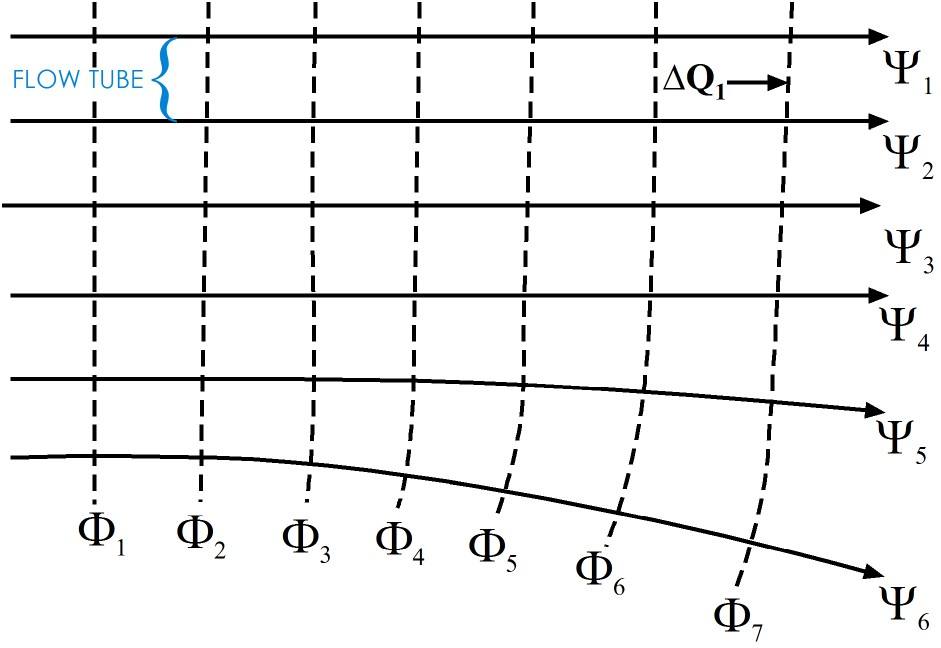
Figure 31 ‑ Sample flow net showing the relationship between gradient and flow tube width. The solid lines (Ψ) are flow lines. The dashed lines (Ф) are equipotentials. [latex]{\Delta Q}_{1}[/latex] is the discharge in one flow tube defined by two flow lines.
When drawing a flow net, the first thing to do is identify the boundary conditions and draw those to scale on the area where the flow net is to be drawn. Usually, when creating a map‑view flow net the flow net will be drawn directly onto a base map; if so, the boundary conditions will likely be readily apparent as indicated by the position of water bodies and low-permeability materials. Boundary conditions must be dealt with as shown in Figure 32a,b, with no-flow boundaries being flow lines and constant head boundaries being equipotential lines.
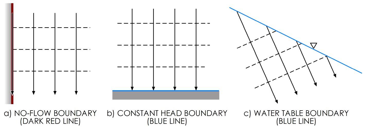
Figure 32 ‑ Rules for dealing with boundaries in a flow net: a) no-flow boundaries are flow lines; b) constant head boundaries are equipotential lines, equipotential lines intersect the water table at the elevation equal to the equipotential line value.
The no‑flow boundary represents a flow line—flow along the boundary is parallel to the boundary, and there is no gradient perpendicular to the boundary. No‑flow boundaries on a flow net represent known flow lines; therefore, those flow lines should be drawn in first and used to constrain subsequent flow lines.
Constant head boundaries, like lakes and streams, are points where the head does not change. For this reason, a constant‑head boundary represents either a single equipotential value (in the case of a lake or pond), or it represents a set of known elevation points (in the case of a stream or river). For lake/pond boundaries, the flow lines always intersect the boundary at right angles, and the nearest equipotentials should be nearly parallel to the boundary. For streams, the equipotentials come into the stream at a tangent—at the point where the line and stream meet, they are parallel. Streams can be difficult to deal with when constructing a rigorous flow net. For simple groundwater contour maps, we need to remember the rules concerning gaining and losing streams. That is, equipotential lines form a vee in the upstream direction for gaining streams, and they form a vee in the downstream direction for losing streams
Water table boundaries (Figure 32c) are often used in constructing a flow net on a cross section. A classic cross‑sectional flow net is flow through an earthen dam (Figure 33).
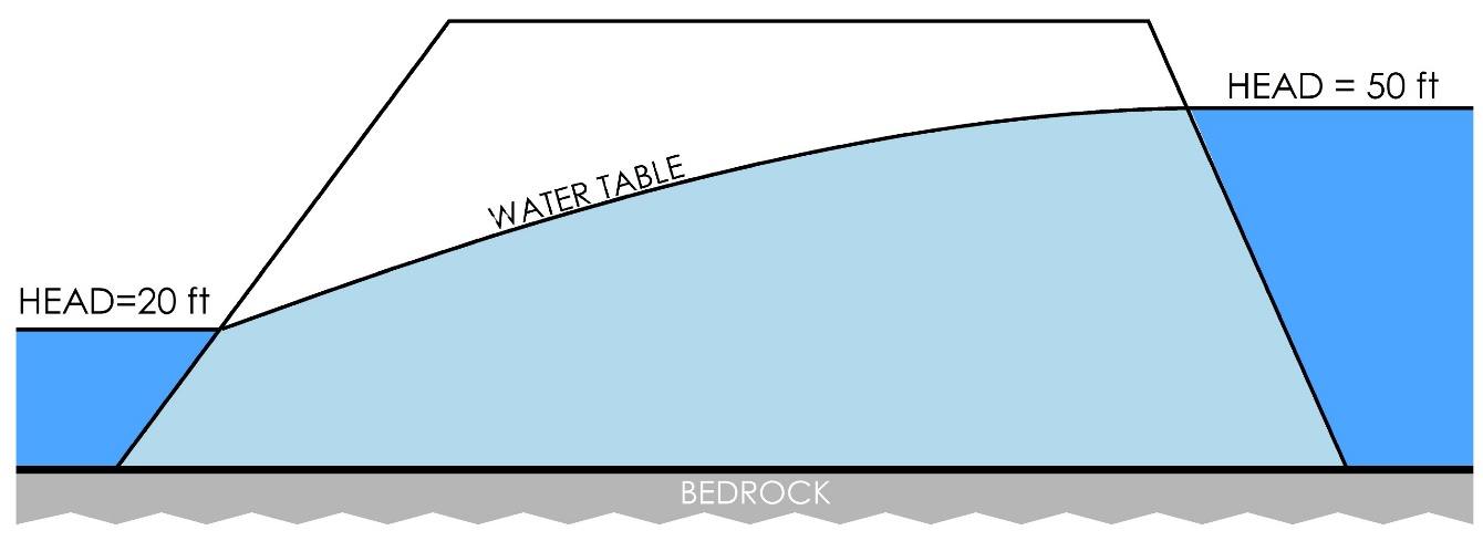
Figure 33 – Cross section showing flow through an earthen dam.
Once the flow net is drawn, the discharge through the flow net can be calculated by the formula shown as Equation (57).
| [latex]q^{1} = \frac{Kdh}{f}[/latex] | (57) |
|---|
where (parameter dimensions are dark green font with mass as M, length as L, time as T):
| [latex]q^{1}[/latex] | = | total volumetric discharge per unit width of aquifer (L3T-1) |
|---|---|---|
| [latex]d[/latex] | = | number of flow tubes (areas bounded by adjacent pairs of flow lines) (:) |
| [latex]h[/latex] | = | total head loss over the length of the flow lines (L) |
| [latex]f[/latex] | = | number of equipotential drops (:) |
If reliable estimates of the total discharge through the flow net are available, then the flow net can potentially be used to estimate the hydraulic conductivity for the aquifer (Exercise 7⮧).
More detailed instructions for constructing flow nets, including examples and exercises, are provided in Graphical Construction of Groundwater Flow Nets↗ by Poeter and Hsieh (2020) which is available from The Groundwater Project as a free download or can be read online.
2 Boundary conditions are discussed in more detail in Section 9