
7.3 Well Hydraulics
Now that we have discussed wells, we discuss how groundwater flows to wells. To understand the hydraulics behind flow to wells, we need to first simplify the system and start with some basic assumptions that are listed here.
- The aquifer is homogeneous and isotropic.
- The aquifer is bounded on the bottom and top by confining layers.
- All geologic formations are horizontal and have infinite horizontal extent.
- The potentiometric surface of the aquifer is horizontal prior to the start of pumping, and water levels are at steady state.
- Any changes to the position of the potentiometric surface are caused only by the pumping well.
- All flow in the aquifer is horizontal.
- All flow to the well is radial.
- Darcy’s law is valid.
- Groundwater has a constant density and viscosity.
- All wells are fully penetrating.
- The diameter of the pumping well is negligible.
Generally, in practice, well hydraulics solutions can be applied even when these assumptions are not rigorously met, but they are needed to be precise with respect to the mathematical development. We now use the groundwater flow equation that we developed in previous sections to describe groundwater flow towards and into a pumping well.
Horizontal Radial Flow
We have discussed and developed the equation that governs the flow of groundwater in three dimensions; as shown by Equation (58).
| [latex]\frac{{\partial q}_{x}}{\partial x} + \frac{{\partial q}_{y}}{\partial y} + \frac{{\partial q}_{z}}{\partial z} = S_{s}\frac{\partial h}{\partial t}[/latex] | (58) |
|---|
where (parameter dimensions are dark green font with mass as M, length as L, time as T):
| q | [latex]=[/latex] | specific discharge (i.e., groundwater flow) in the [latex]x,\ y,[/latex] or [latex]z[/latex] direction (LT‑1) |
|---|---|---|
| x, y, z | [latex]=[/latex] | lengths in the principal directions in our coordinate systems |
| [latex]h[/latex] | [latex]=[/latex] | hydraulic head (L) |
| [latex]t[/latex] | [latex]=[/latex] | time (T) |
| [latex]S_{s}[/latex] | [latex]=[/latex] | specific storage (L‑1) |
We substituted Darcy’s law—shown as Equation (59)—for q.
| [latex]q = - K\frac{dh}{dl}[/latex] | (59) |
|---|
where (parameter dimensions are dark green font with mass as M, length as L, time as T):
| [latex]K[/latex] | = | hydraulic conductivity (LT-1) |
|---|---|---|
| [latex]\frac{dh}{dl}[/latex] | = | hydraulic gradient, or change in head with distance, l ([latex]:[/latex]) |
The result is Equation (60).
| [latex]\frac{\partial\left( K_{x}\frac{\partial h}{\partial x} \right)}{\partial x} + \frac{\partial\left( K_{y}\frac{\partial h}{\partial y} \right)}{\partial y} + \frac{\partial\left( K_{z}\frac{\partial h}{\partial z} \right)}{\partial z} = S_{s}\frac{\partial h}{\partial t}[/latex] | (60) |
|---|
Now, if we assume the aquifer is homogeneous and isotropic (as discussed in Section 5—More on Flow Equations), but not necessarily steady‑state, the result appears as Equation (61).
| [latex]K\left( \frac{\partial^{2}h}{{\partial x}^{2}} + \frac{\partial^{2}h}{{\partial y}^{2}} + \frac{\partial^{2}h}{{\partial z}^{2}} \right) = S_{s}\frac{\partial h}{\partial t}[/latex] | (61) |
|---|
Assumption #6 states that all flow is horizontal. This means that there is no vertical component of flow, and therefore, the [latex]z[/latex] term can be eliminated to obtain Equation (62).
| [latex]K\left( \frac{\partial^{2}h}{{\partial x}^{2}} + \frac{\partial^{2}h}{{\partial y}^{2}} \right) = S_{s}\frac{\partial h}{\partial t}[/latex] | (62) |
|---|
Now, recalling that transmissivity ([latex]T[/latex]) is defined as [latex]T = Kb[/latex] (where [latex]b[/latex] is the saturated thickness of the aquifer) and storativity ([latex]S[/latex]) is defined as[latex]\ S = S_{s}b[/latex], we multiply both sides by [latex]b[/latex], to get Equation (63).
| [latex]Kb\left( \frac{\partial^{2}h}{{\partial x}^{2}} + \frac{\partial^{2}h}{{\partial y}^{2}} \right) = S_{s}b\frac{\partial h}{\partial t}[/latex] | (63) |
|---|
Then, substituting with S and T, and dividing both sides by T, we obtain Equation (64).
| [latex]\frac{\partial^{2}h}{{\partial x}^{2}} + \frac{\partial^{2}h}{{\partial y}^{2}} = \frac{S}{T}\frac{\partial h}{\partial t}[/latex] | (64) |
|---|
If the aquifer is receiving recharge, either from infiltration of rain in an unconfined aquifer, or from leakage through a confining layer in a confined aquifer, we can add that directly to the equation and get Equation (65).
| [latex]\frac{\partial^{2}h}{{\partial x}^{2}} + \frac{\partial^{2}h}{{\partial y}^{2}} + \frac{w}{T} = \frac{S}{T}\frac{\partial h}{\partial t}[/latex] | (65) |
|---|
where (parameter dimensions are dark green font with mass as M, length as L, time as T):
| [latex]w[/latex] | = | rate of vertical leakage or recharge (LT‑1) |
|---|
Now, the thing about flow to a well is that it is radial; in other words, flow lines are converging on the well from all sides (Figure 36). Because the flow lines converge, the equipotential lines—indicated by dashed lines on Figure 36 get closer together near the well. This represents the cone of depression that forms around the well.
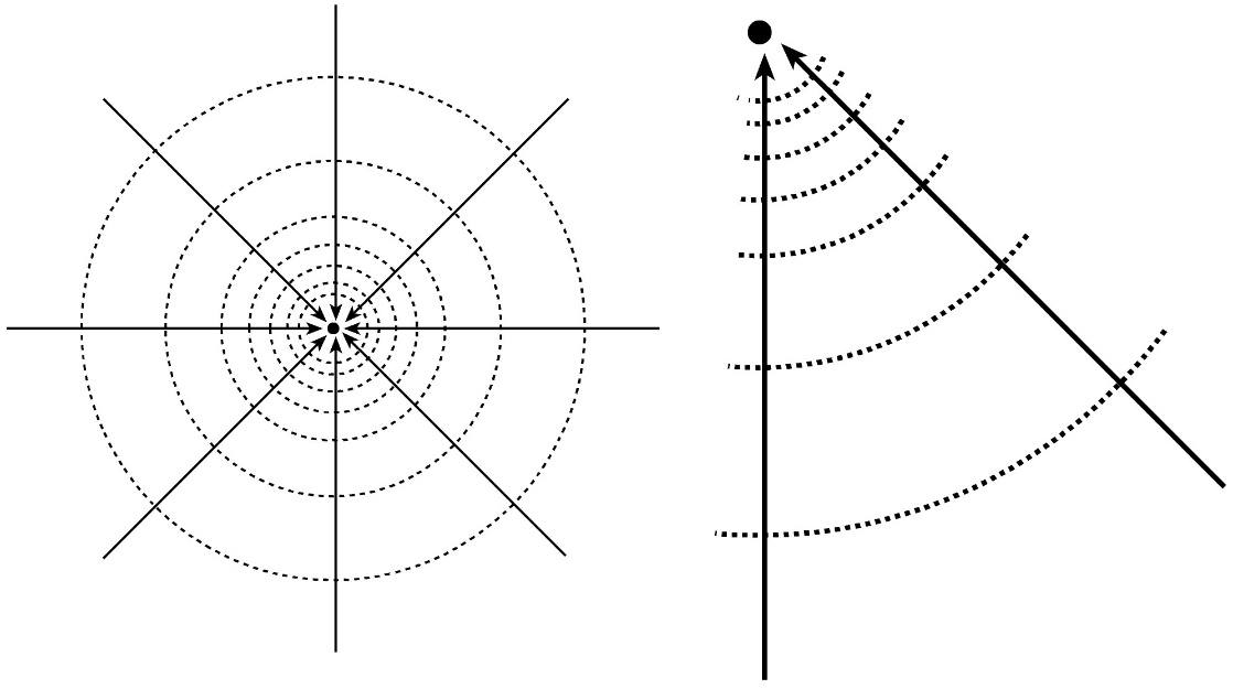
Figure 36 ‑ Radial flow to a well. The dashed lines are equipotential lines that are lowest closest to the well, which is represented by the dot in the center.
Now, because we are dealing with radial flow to the well, it helps to express the equations in terms of a polar (or cylindrical) coordinate system rather than the simple Cartesian ([latex]x,\ y[/latex]) coordinate system. In polar coordinates, a point is defined by its location with respect to a fixed central pole (in this case, the well). The location of a point is defined by its radial distance from the pole ([latex]r[/latex]) and the angle ([latex]\theta[/latex]) between the radial line and some fixed polar axis (for example, north). Polar coordinates are graphically described in Figure 37.
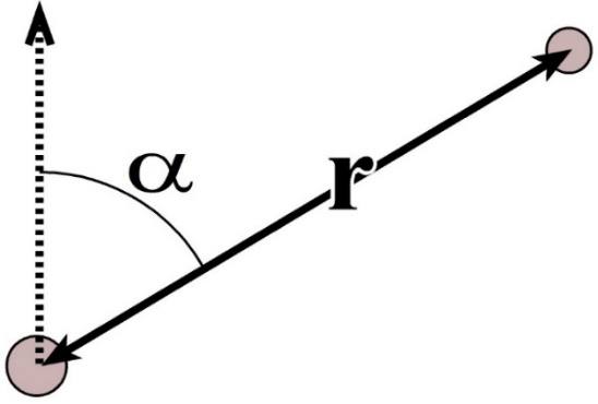
Figure 37 ‑ Polar coordinate system.
We can use the Pythagorean Theorem and some basic geometry to re‑state our two‑dimensional flow equations in polar coordinates (Box 1⮧ shows a complete derivation). When we do so, we have Equation (66) and Equation (67).
| [latex]\frac{\partial^{2}h}{{\partial r}^{2}} + \frac{1}{r}\frac{\partial h}{\partial r} = \frac{S}{T}\frac{\partial h}{\partial t}[/latex] | (66) | |
|---|---|---|
| [latex]\frac{\partial^{2}h}{{\partial r}^{2}} + \frac{1}{r}\frac{\partial h}{\partial r} + \frac{w}{T} = \frac{S}{T}\frac{\partial h}{\partial t}[/latex] | (67) |
Equation (67) is a differential equation that describes radial horizontal flow to a well based on a polar coordinate system. Since it is a differential equation, it requires some complex mathematical operations—like Fourier transforms, Bessel functions, and Laplace transforms—to solve. Fortunately for us, these solutions have already been done, and all you need at this point is some understanding of what they mean and how they are used.