
7.4 The Theis Equation
In Section 3, we discussed that the mathematics governing the flow of groundwater—that is, the mathematics showing that groundwater discharge is proportional to a gradient—are identical to those that govern many other physical processes like the flow of heat in a solid, the diffusion of solutes in solution, and electrical current through a conductive solid. In the 1930s a civil engineer, C. V. Theis, noted the similarity between groundwater flow and heat flow, and he noted that pumping a well was mathematically analogous to heating a block of metal with a thermally conductive rod (Figure 38).
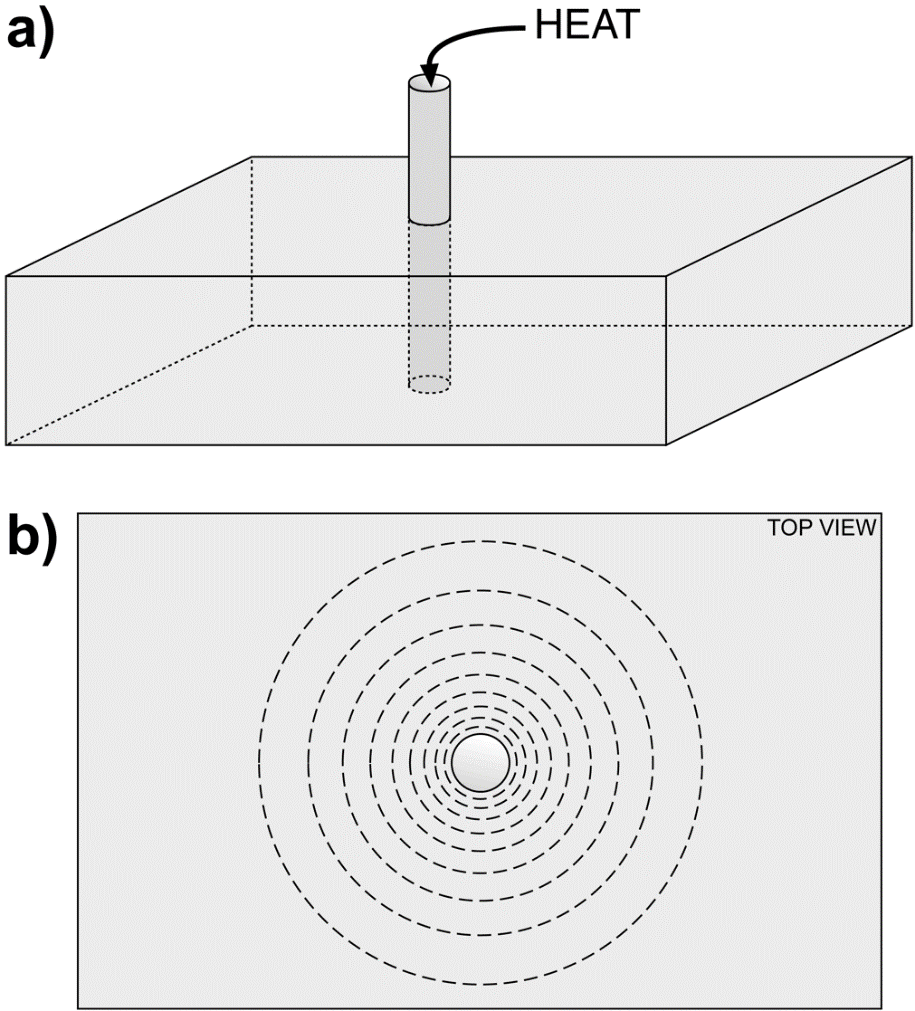
Figure 38 a) Metal rod heating a metal plate, and b) contour lines of equal temperature with higher temperature near the rod.
This situation assumes that the block has a constant thickness and an infinite extent—even though it is drawn here as a block with finite proportions. If we start with the block at a constant temperature, then begin to heat the rod with a constant temperature, heat will be transferred to the block. It will take time for heat to move through the block, and the rate of movement of heat is dependent upon the thermal conductivity of the metal.
The part of the block immediately adjacent to the rod will heat up first, then heat will flow through the block and, over time develop a distribution of temperatures like the contours shown in Figure 38b. Conversely, if we start with a warm block of metal and cool the end of the rod, heat will flow out of the metal into the rod and set up a similar distribution of temperatures with lower values near the rod. Mathematically this is the same thing that happens in an aquifer pumped by a well, except that water is flowing instead of heat, and a distribution of heads form instead of a distribution of temperatures. That distribution of heads in an aquifer is the cone of depression.
Theis (1935) developed this idea mathematically as shown in Equation (68).
| [latex]s = \frac{Q}{4\pi T}W(u)[/latex] | (68) |
|---|
The value of u is defined in Equation (69).
| [latex]u = \frac{r^{2}S}{4Tt}[/latex] | (69) |
|---|
[latex]W(u)[/latex] is the well function, which is the integral of [latex]u[/latex] from [latex]u[/latex] to infinity, as shown in Equation (70).
| [latex]W(u) = \int_{u}^{\infty}\frac{e^{- u}du}{u}[/latex] | (70) |
|---|
[latex]W(u)[/latex]can also be expressed as the infinite series in Equation (71).
| [latex]W(u) = - 0.5772 - \ln{u + u - \frac{u^{2}}{2*2!}} + \frac{u^{3}}{3*3!} - \frac{u^{4}}{4*4!} + \frac{u^{5}}{5*5!} - and\ so\ on\ldots[/latex] | (71) |
|---|
where (parameter dimensions are dark green font with mass as M, length as L, time as T):
| [latex]s[/latex] | [latex]=[/latex] | drawdown (L), defined as the initial head minus the head at time [latex]t[/latex] |
|---|---|---|
| [latex]Q[/latex] | [latex]=[/latex] | pumping rate from the well (L3T-1); assumed to be constant |
| [latex]T[/latex] | [latex]=[/latex] | aquifer transmissivity (where [latex]T\ = \ Kb[/latex]) (L2T-1) |
| [latex]r[/latex] | [latex]=[/latex] | radius (distance from pumping well) (L) |
| [latex]S[/latex] | [latex]=[/latex] | storativity (where [latex]S\ = \ S_{s}b[/latex]) (:) |
| [latex]t[/latex] | [latex]=[/latex] | time after the start of pumping ([latex]T[/latex]) |
An important thing to note at this point is that we are describing a transient situation; in other words, we are interested in understanding how heads in an aquifer change with respect to time when water is pumped from a well at a constant rate. That is what the Theis equation calculates—the drawdown at a point in the aquifer some distance from the pumping well ([latex]r[/latex]) at some time ([latex]t[/latex]) after pumping begins in response to a well pumping at a constant rate ([latex]Q[/latex]). If one knows the transmissivity and storativity of a confined aquifer, then the equation can be used to predict how much drawdown a pumping well will generate in that aquifer at some distance from the pumping well and at some time after the start of pumping (Exercise 8⮧).
Solving the Theis equation requires values of [latex]W(u)[/latex] for corresponding values of u. A table of values of [latex]W(u)[/latex] for values of [latex]u[/latex] is provided as Table 4 (Exercise 9⮧).
Table 4 ‑ Values of W(u) for values of u. For example, for u=4×10⁻⁷, W(u)=14.15.
| u | 1.0 | 2.0 | 3.0 | 4.0 | 5.0 | 6.0 | 7.0 | 8.0 | 9.0 |
| 1×10‑0 | 0.219 | 4.9×10‑2 | 1.3×10‑2 | 3.8×10‑3 | 1.1×10‑3 | 3.6×10‑4 | 1.2×10‑4 | 3.8×10‑5 | 1.2×10‑5 |
| 1×10‑1 | 1.82 | 1.22 | 0.91 | 0.70 | 0.56 | 0.45 | 0.37 | 0.31 | 0.26 |
| 1×10‑2 | 4.04 | 3.35 | 2.96 | 2.68 | 2.47 | 2.30 | 2.15 | 2.03 | 1.92 |
| 1×10‑3 | 6.33 | 5.64 | 5.23 | 4.95 | 4.73 | 4.54 | 4.39 | 4.26 | 4.14 |
| 1×10‑4 | 8.63 | 7.94 | 7.53 | 7.25 | 7.02 | 6.84 | 6.69 | 6.55 | 6.44 |
| 1×10‑5 | 10.94 | 10.24 | 9.84 | 9.55 | 9.33 | 9.14 | 8.99 | 8.86 | 8.74 |
| 1×10‑6 | 13.24 | 12.55 | 12.14 | 11.85 | 11.63 | 11.45 | 11.29 | 11.16 | 11.04 |
| 1×10‑7 | 15.54 | 14.85 | 14.44 | 14.15 | 13.93 | 13.75 | 13.60 | 13.46 | 13.34 |
| 1×10‑8 | 17.84 | 17.15 | 16.74 | 16.46 | 16.23 | 16.05 | 15.90 | 15.76 | 15.65 |
| 1×10‑9 | 20.15 | 19.45 | 19.05 | 18.76 | 18.54 | 18.35 | 18.20 | 18.07 | 17.95 |
| 1×10‑10 | 22.45 | 21.76 | 21.35 | 21.06 | 20.84 | 20.66 | 20.50 | 20.37 | 20.25 |
| 1×10‑11 | 24.75 | 24.06 | 23.65 | 23.36 | 23.14 | 22.96 | 22.81 | 22.67 | 22.55 |
| 1×10‑12 | 27.05 | 26.36 | 25.96 | 25.67 | 25.44 | 25.26 | 25.11 | 24.97 | 24.86 |
| 1×10‑13 | 29.36 | 28.66 | 28.26 | 27.97 | 27.75 | 27.56 | 27.41 | 27.28 | 27.16 |
| 1×10‑14 | 31.66 | 30.97 | 30.56 | 30.27 | 30.05 | 29.87 | 29.71 | 29.58 | 29.46 |
| 1×10‑15 | 33.96 | 33.27 | 32.86 | 32.58 | 32.35 | 32.17 | 32.02 | 31.88 | 31.76 |