
9.2 Characteristics of Flow Systems
A groundwater flow system is a three‑dimensional entity with the following components:
- volume and boundary conditions: dimensions encompassing a finite volume and physical boundaries to flow;
- recharge: an area and set of processes that allow water to enter; and
- discharge: an area and set of processes that allow water to exit.
- Next, we discuss each of these components.
Boundary Conditions
Flow systems are three dimensional bodies that have physical boundaries. There are two basic types of boundaries, or boundary conditions, that we use to characterize the limits of flow systems: specified flux (or Neumann) boundary—in particular the special case of no-flow; and specified head (or Dirichlet)—in particular the special case of constant head). Other types of boundaries are variations and combinations of the Neumann and Dirichlet boundaries that get their names from people who first described them.
No‑Flow Boundaries
A no‑flow boundary is a boundary that possesses qualities that do not allow for the flow of groundwater across the boundary. It is a special case of a specified flux boundary with zero flux. Since there is no flow across the boundary, there is also no hydraulic gradient across the boundary—that is, [latex]dh/dx\ = 0\ ,[/latex] where [latex]x[/latex] is perpendicular to the boundary. Some examples are provided here.
- If permeable aquifer units are directly in contact with low‑permeability formations—for example, alluvial deposits adjacent to an upthrown block of granite or other low‑[latex]K[/latex] crystalline rock at a fault—then there will be no significant flow from the low‑[latex]K[/latex] rock into the flow system, or vice versa (Figure 59). This is the same as the situation described in Figure 55 and Figure 56a.
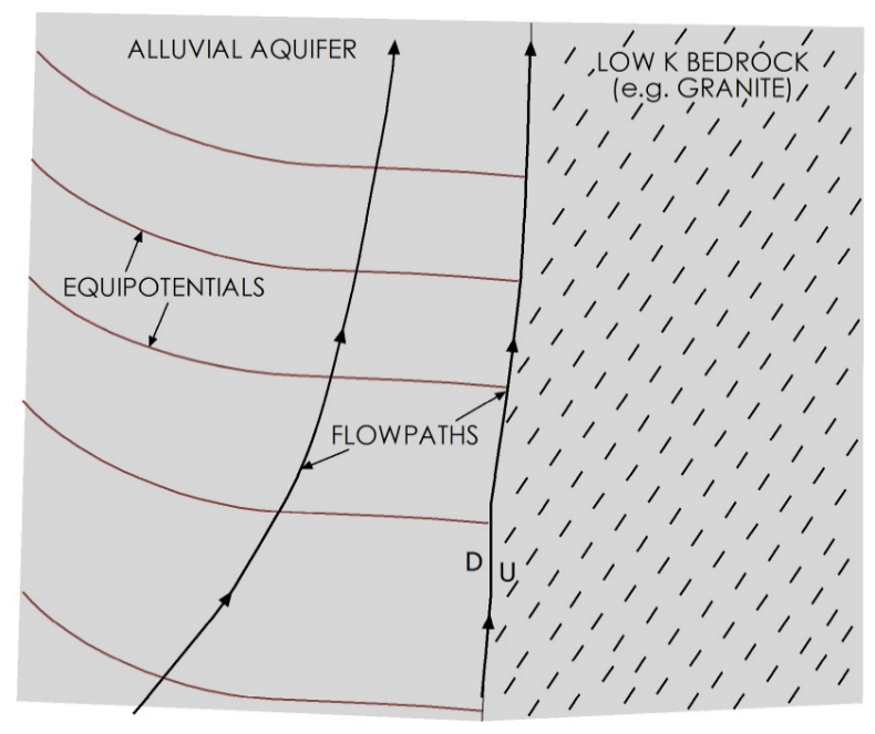
Figure 59 ‑ No‑flow boundary.
- Locally high groundwater levels can produce a groundwater divide—analogous to a surface water or watershed divide. At a groundwater divide, all hydraulic gradients—and groundwater flow—are away from the boundary; therefore, there is no hydraulic gradient or flow perpendicular to the boundary (Figure 60). Since flow is moving away from the boundary, water must be coming into the flow system at that point; therefore, groundwater divides are typically associated with recharge areas.
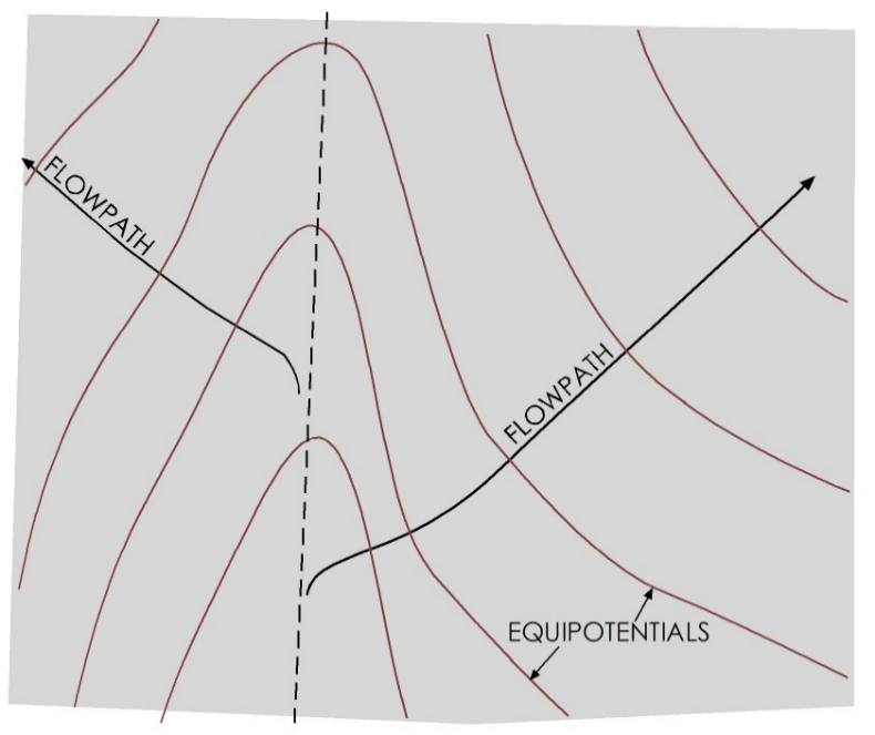
Figure 60 ‑ No‑flow boundary at a groundwater divide.
- Wherever parallel flow lines exist in an aquifer, there is no hydraulic gradient, and therefore no flow occurs in the direction perpendicular to the flow lines. This case is called a symmetry boundary (Figure 61).
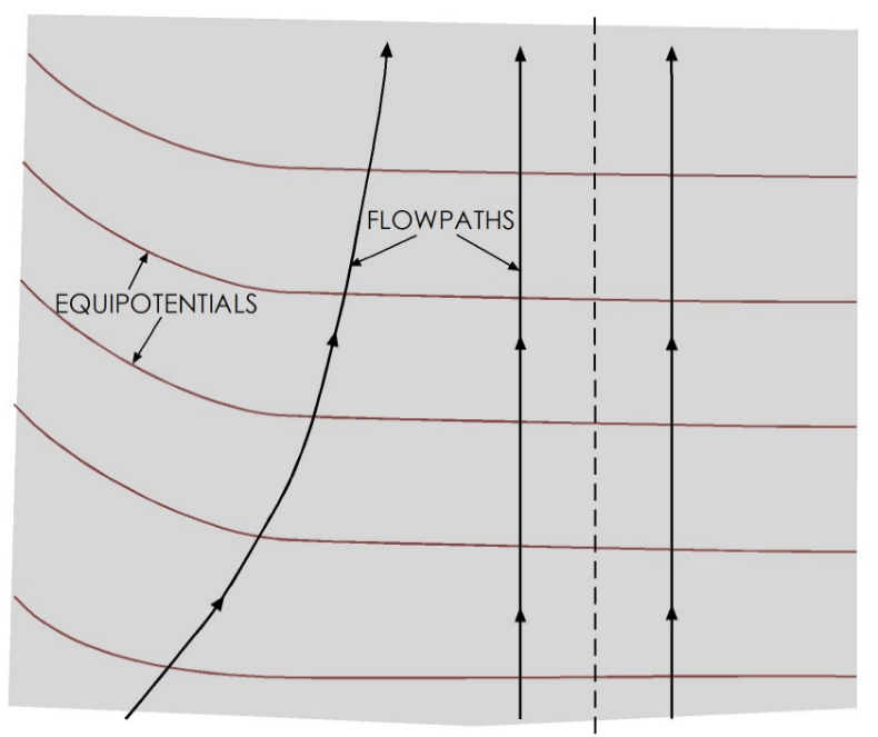
Figure 61 ‑ No‑flow symmetry boundary.
Constant Head
A constant head boundary is a boundary at which the hydraulic head within the aquifer does not change. It is a special case of a specified head boundary with unchanging head. Constant head boundaries form where a groundwater flow system is in direct hydraulic communication with a body of surface water that has a constant water level. At the boundary, the hydraulic head in the groundwater system is equal to the water level elevation in the surface water body. An example of this is along the coast of a non‑flowing body of water—for example, a lake or a pond—such as that depicted in Figure 62. In this case, the shore of the lake represents a single equipotential line within the aquifer that is equivalent to the elevation of the lake surface. If the water levels in the groundwater flow system are greater than those in the lake, then water will flow into the lake perpendicular to the shoreline.
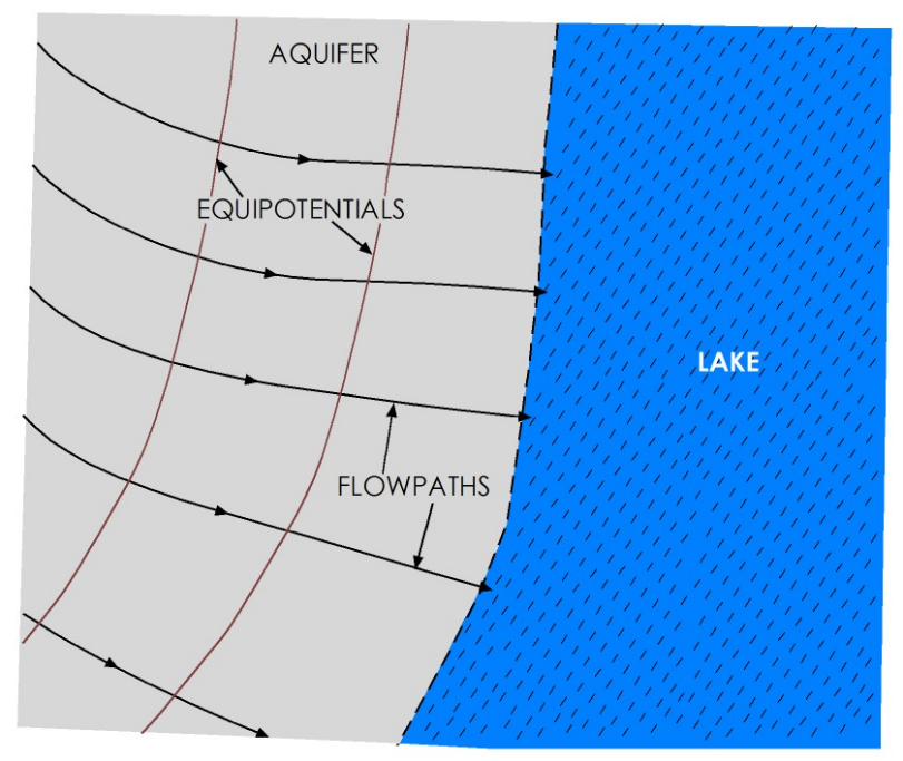
Figure 62 ‑ Constant head boundary at a lake.
If the boundary is along a river, the heads will vary along the length of river as its stage decreases downstream, but at any point along the stream channel the heads in the aquifer are equivalent to the river stage at that point. Each point along the river therefore represents a point on an equipotential line in the groundwater flow system (Figure 63). It should be noted that, as lake and river stage elevations change in response to droughts or large precipitation events, the heads within the groundwater at the boundary do so too.
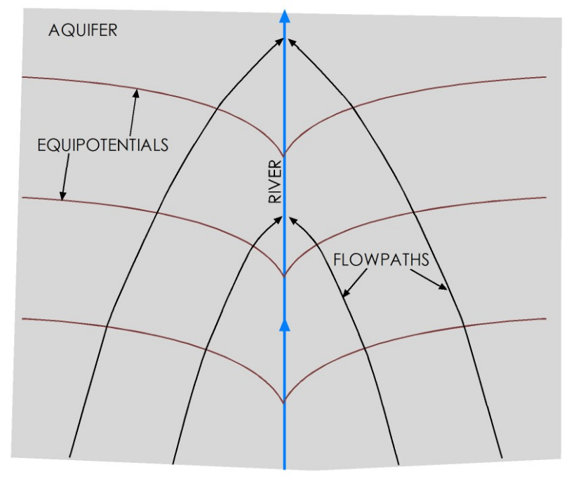
Figure 63 ‑ Constant head boundary along a gaining stream.
Other Boundary Conditions
The two boundary conditions presented in this section represent the boundaries most frequently dealt with in understanding groundwater flow systems. Other boundary conditions exist, including head‑dependent flux (Cauchy) boundary, Robin boundary (a weighted sum of Neumann and Dirichlet conditions), Mixed boundary (with varying boundary types along its length), a free-surface boundary that describes a water table or salt-water interface, and a seepage face boundary that is a free-surface boundary confined to a plane on the earth’s surface. A discussion of these is beyond the scope of this book.
Recharge
Recharge refers to the set of processes by which water enters the saturated part of a groundwater flow system. Areas where recharge is occurring are called recharge areas or recharge zones. There are several ways that recharge gets into a flow system.
- Direct infiltration on the outcrop with some percentage of rainwater seeping into the ground and ultimately flowing through the water table into the saturated zone.
- Infiltration through the beds of losing streams or reservoirs. In some parts of the world, especially in extremely arid regions, this is the dominant form of recharge to the groundwater.
- Interformational flow, or subsurface flow, from one formation/flow system directly into another system, usually as flow through leaky confining layers or zones where two flow systems are in direct hydraulic communication.
The primary source of water for recharge is precipitation. When it rains, some percentage of the water runs off over the surface, some evaporates back into the atmosphere, some is taken up by plants and animals (transpiration), and the remainder gets to the water table and recharges the aquifer. In addition, some amount of surface runoff may flow into and through surface water bodies that are actively losing water to the underlying groundwater system. Finally, accumulation of snow at higher elevations in winter can result in additional surface water flow and recharge during spring thaw. Recharge is therefore frequently quantified as some percentage of precipitation. We can measure precipitation in a given area with a high level of confidence. We can also measure stream discharge and runoff and get a good estimate of how much of a rainstorm ends up as runoff. We can measure potential evaporation by placing a pan of water outside and seeing how long it takes to evaporate. However, it is more difficult to estimate transpiration and actual evaporation. Transpiration is difficult to quantify because any given area has a wide range of plants, and the overall transpiration is a function of the various percentages of each type of plant present in the area. Actual evaporation is difficult to quantify because it depends upon how much water is available on the surface at any given time; plus, evaporation rates vary with conditions such as temperature, humidity, windspeed, and solar radiation. Because of the many processes involved and uncertainties associated with their magnitudes, it is always difficult to put a number on recharge to any aquifer. Generally, it is accepted that annual recharge rates in most aquifers are somewhere between 1 and 10 percent of annual precipitation, though it can be as high as 30 percent in humid regions.
Discharge
Discharge is the set of processes by which water leaves the saturated part of a groundwater flow system. Discharge processes include:
- discrete discharge to a spring or seep;
- discharge into a gaining stream, wetland, or lake;
- interformational flow (leakage through a confining layer);
- evaporation—in some arid areas, this is the primary mechanism for discharge from flow systems; and
- pumping from a well.
Discharge can also be difficult to quantify, especially in areas dominated by well pumping or evaporation. Interformational flow is generally small compared to the other mechanisms. Springs and gaining streams can be gaged, and changes in their flow can be attributed to either recharge or discharge. Much of the discharge from actively developed aquifers is via pumping from wells, and many aquifers suffer from a lack of reliable records for volumes of water pumped over time.
Readers who are interested in learning more about recharge and discharge processes, specifically those associated with the interactions between groundwater and surface water, are encouraged to download and review Groundwater‑Surface Water Exchange↗ by Woessner (2020) which is available from The Groundwater Project as a free download or can be read online.
Heterogeneity and Anisotropy
Heterogeneity refers to variations in the characteristics of a system with respect to location. A parameter like permeability will vary from place to place in a flow system, depending upon the rock types and variations in sediment characteristics—such as grain size. A common example of heterogeneity in a flow system is interbedded sand and clay units in a fluvial depositional system.
Heterogeneity affects flow paths in two ways. One, if the interface between the different zones is parallel to the flow directions, water will tend to move in the path of least resistance. This affects the localized flow paths water takes in a system; for example, in Figure 64 the overall direction of flow is left to right on the diagram, but in some areas the heterogeneity results in flow lines with vertical components.
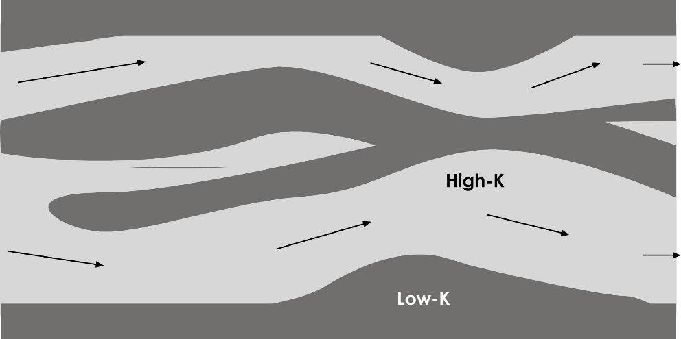
Figure 64 ‑ Influence of heterogeneities on flow paths.
The second way that heterogeneity affects flow directions is associated with refraction of flow lines at the boundaries between units with different hydraulic conductivities. When groundwater moves from a formation with a given hydraulic conductivity into a formation with a different conductivity, the discharge between each flow lines stays the same. However, since [latex]K[/latex] is different, the gradient must change, and therefore the flow lines must move either together or apart, depending on whether the change in [latex]K[/latex] is increasing or decreasing. Therefore, when flow lines cross into areas with different conductivities, they refract or bend—like light moving through a substance with one optical velocity into one with a different optical velocity. If the conductivities of the two formations are known, the angles of refraction can be calculated using Equation (88) with [latex]K[/latex] and [latex]\alpha[/latex] defined in Figure 65.
| [latex]\frac{K_{1}}{K_{2}} = \frac{\tan\left( \alpha_{1} \right)}{\tan\left( \alpha_{2} \right)}[/latex] | (88) |
|---|
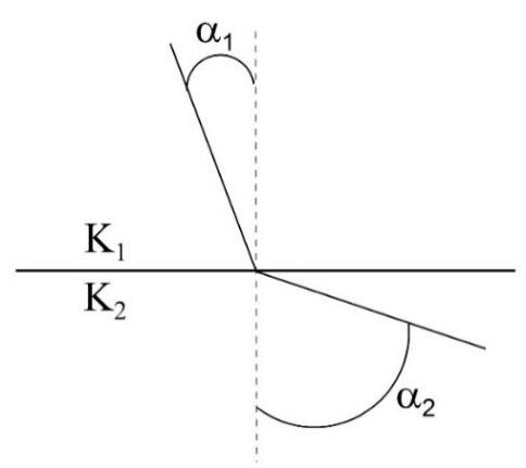
Figure 65 ‑ Refraction of flow lines at the interface of two formations with different conductivities.
The amount of refraction, and the direction in which the flow lines are refracted—relative to the line normal to the interface—is determined by the degree of difference in hydraulic conductivity and by which way the water is flowing (Figure 66).
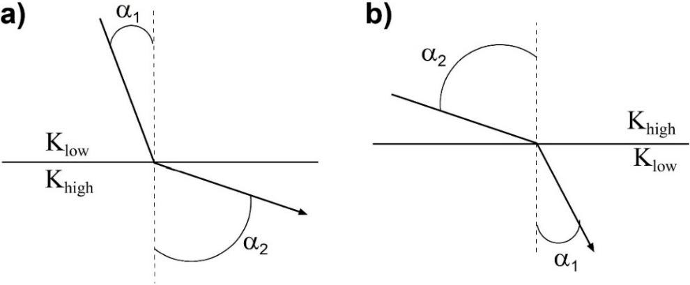
Figure 66 ‑ Refraction of flow lines a) low to high conductivity; b) high to low conductivity.
As a result, low permeability formations tend to have vertical gradients and vertical flow, whereas higher permeability formations tend to have horizontal flow lines. In a layered system of interbedded sand and clay, the horizontal permeability will be much greater than the vertical permeability, and as a result, in layered systems the overall flow direction tends to be horizontal direction and concentrated in the higher [latex]K[/latex] units. Flow in lower [latex]K[/latex] units tends to be vertical (Figure 67).
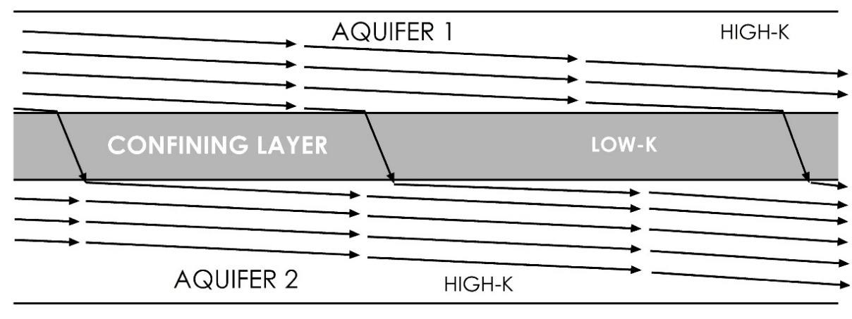
Figure 67 ‑ Cross‑section showing effect of heterogeneity in the form of layered sediments on flow paths which creates anisotropy for the system of layers.
Anisotropy refers to variations with respect to direction. Layering of interbedded high and low [latex]K[/latex] formations, as shown in Figure 67, is one form of anisotropy. Anisotropy can also result from sedimentary structures formed during deposition, both on a large scale—like channel sands interspersed with overbank deposits in a fluvial system—and on a smaller scale—cross‑beds, graded bedding. More significantly, geologic structures like fractures are frequently responsible for anisotropic aquifers.
As shown in Figure 30, if the direction of maximum permeability in an anisotropic system is not parallel to the gradient, the flow paths will be deflected and will not follow the gradient. In moderately anisotropic aquifers, a groundwater map showing the equipotentials does not indicate the primary flow directions. For example, in the Edwards Aquifer of central Texas the overall hydraulic gradient points towards the Gulf Coast. However, extensive fracturing associated with the Balcones Fault Zone, and later karstification, has created an anisotropy that deflects the flow paths so that they are almost parallel to the equipotentials. For more information, The Edwards Aquifer↗ by Sharp and Green (2022) is available as a free download from The Groundwater Project as a free download or can be read online.
Relationship between Topography and Flow Systems
King (1899) and Hubbert (1940) noted the relationship between topography and groundwater flow patterns. Both noticed that the water table tends to be a subdued replica of the topography (Figure 68).
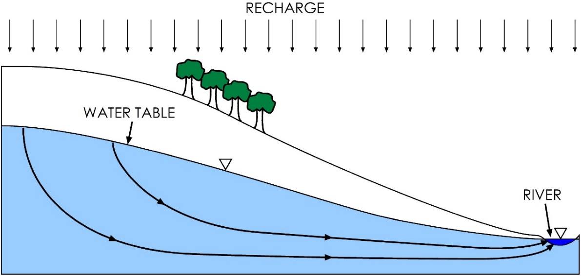
Figure 68 ‑ Cross section of water table aquifer showing the relationship between topography and the orientation of the water table.
Tóth (1963) then developed a computer model, using the same groundwater flow equations that we presented in the previous sections. This is important because Tóth’s model was one of the first numerical computer groundwater models and it paved the way for a lot of later groundwater modeling approaches and techniques. His model looked at how flow systems are related to topography. He set up his model as a two‑dimensional cross section and used a mathematical equation to define a specified head boundary that represented a water table mimicking uneven topography on the surface. When he varied the topography, he noted that, in some places, smaller local flow systems would develop within the larger regional flow systems. This was the first mathematical evidence that these types of systems exist, and it confirmed the findings of King and Hubbert. Exercise 18⮧ provides an opportunity to create a representation of a topographically driven flow system and track groundwater flowlines and particles through the system.
The relationship between topography and groundwater flow patterns is generally only valid in humid areas with sufficient rainfall to support recharge to the water table. For example, Uliana (2000) used naturally occurring isotopes and major ion chemistry, in conjunction with analytical modeling to show that regional groundwater flow patterns in a subtropical arid region (the Chihuahuan desert of west Texas, USA) flow beneath one of the mountain systems and cross the surface drainage divides.