
10.2 Models: A General Definition and Specific Details
There are a lot of different definitions of the word model; so many that I came up with my own. A model is a simplified representation of an object, structure, or process that cannot be studied directly because it is too large, too small, or too complicated, or because direct study or observation is, for other reasons, not possible or feasible.
One of the keys to this definition is that we can represent a process as well as a structure or object. We traditionally think of models in the sense of things that represent the structure or appearance of something, like a plastic model airplane or a stick model of a benzene molecule. Model airplanes can be very sophisticated in their representation of the appearance and detail of a real airplane—everything is scaled down correctly, and the details can even include the rivets on the wing and the instrumentation in the cockpit. It is important to recognize, however, that the model just looks like a plane; it can’t actually act like a plane—that is, it can’t fly. The model of an organic molecule is the same—it may have the correct bond angles and the relative size of the atoms is correct, but it does not exhibit the same behavior as a real molecule—for example, it doesn’t bond with other molecules, it doesn’t have a melting or boiling point. These types of models are called geometric models because they depict the geometry—that is, structure, appearance, distribution, etc.—of whatever it is they represent. Some examples of geometric models are:
- plastic toy figures of WWII fighter planes;
- blueprints;
- geologic maps and cross sections; and
- molecular symbols and diagrams (Figure 69).
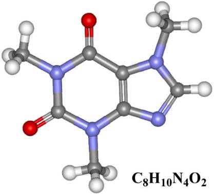
Figure 69 ‑ A model of the author’s favorite molecule.
It is of more importance to us as scientists and hydrogeologists to be able to develop process models, or models that simulate physical processes. These models must contain some component of the geometry of the system, but they also have some component that describes how the system behaves—that is, how it responds to changes in certain conditions, how it changes with time, and so on. This component can be a physical object, or it could be purely mathematical—that is, an equation or a set of equations.
Process models can simulate objects and processes such as the examples listed here.
- Weather and climate
- Make forecasts about weather conditions in the near future.
- Simulate the response of global climate to changes in atmospheric [latex]{CO}_{2}[/latex].
- Stress and strain
- Simulate stresses in a bridge or building foundation.
- Simulate strain in deformed geologic units.
- Watersheds
- Simulate flooding in response to large storms.
- Calculate flow rates at various points in watershed.
- Aquifers and groundwater flow systems
- Simulate changes in head with response to pumping.
- Calculate well yields and long‑term availability.
Why Do We Use Process Models?
The main reasons for developing and using process models for groundwater flow systems—as well as other natural phenomena—are outlined below.
Make Predictions
Forecasting and making predictions about the future state of a system is the most common and most widely recognized reason for developing process models. More specifically, groundwater flow models are widely used to make predictions, generally about how the system will change in the future in response to a change or a stress applied to it. One example of a change to a groundwater system could be reduction in precipitation, and a corresponding reduction in recharge, in response to future climate change. An example of a stress applied to a groundwater system could be the addition of a large amount of pumping associated with a proposed industrial development. These models can be very useful tools for managing water resources; however, one must always remember that models are only as good as the data and assumptions used to develop them, and caution must always be taken when making management decisions based on model predictions.
Test Hypotheses and Investigate Processes
In some cases, we may not be sure why a natural process behaves the way it does, and a model can help us constrain our hypotheses concerning that behavior. For example, we may be studying the structure of a set of folded and faulted rocks. We don’t know exactly what stresses caused the strain that we observe, so we develop hypotheses about compression and tension and the principal stress directions. We then put together a model that simulates those stresses and compare the model results to the structure of the rock in the field. If the model results don’t match, then we need to refine or reformulate the hypotheses. If the model results do match, then the model supports the hypotheses. Keep in mind when model results match field observations it doesn’t prove anything; however, model results can provide robust support for a hypothesis when models are properly developed.
Evaluate System Sensitivity
Another use of models is to help the investigator identify areas where more data is needed. Models can be used to test the sensitivity of a system to certain parameters, and a model may show that the variations of one parameter don’t make much difference in system behavior, while variation of another parameter makes a big difference. For example, a hydrogeologist designing a model for evaluating groundwater pumping from a regional aquifer may have a lot of reliable transmissivity values from several single well aquifer tests but only a few storativity values. A sensitivity analysis of the aquifer may indicate that the model results do not vary much over the range of available storativity estimates, which means that the model results are acceptable and there is likely no need to perform additional aquifer tests to improve the model results.
Estimate Parameters (Inverse Models and Model Calibration)
If we know a lot about our system but are uncertain about the values of a specific parameter, we can use a model to estimate that parameter by applying the information that we know and solving for what we don’t know. Models developed for the purpose of estimating input parameters are called inverse models. Figure 70 and Figure 71 provide an example of simple inverse modeling to estimate a representative transmissivity for a regional groundwater flow system. Using the calculations shown in Figure 70 with the system parameters outlined in Figure 71, along with recharge values ranging from 0.5 to 5 percent of annual precipitation, results in transmissivity values ranging from 1.07 m2/s to 10.7 m2/s. These values are within the range of values estimated from aquifer tests and other methods for the area shown in Figure 71.
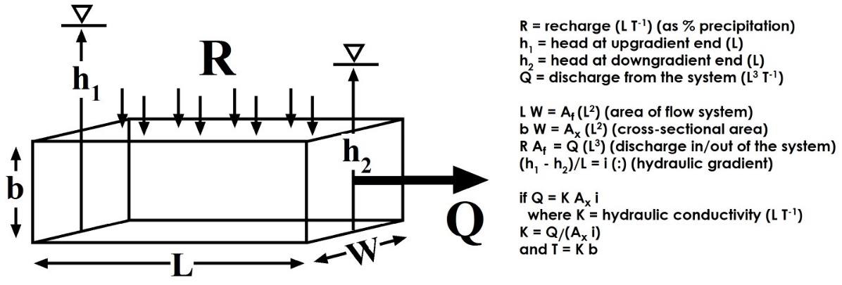
Figure 70 ‑ Schematic diagram illustrating inverse model determination of transmissivity (after Uliana, 2000).
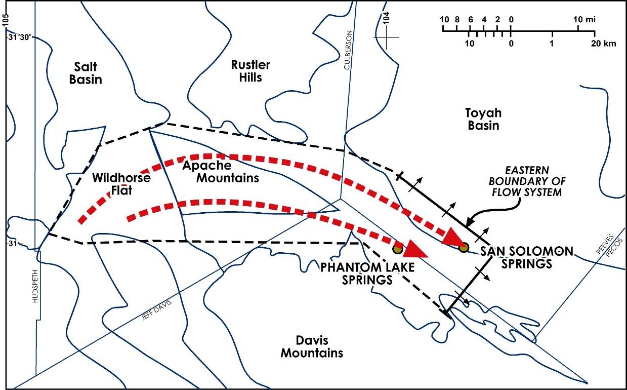
Figure 71 ‑ Map of an area used in regional transmissivity and residence time calculations. The polygon enclosing the regional flow system (dashed lines) has an approximate area of 240 square kilometers. The solid line north and east of the springs represents the eastern boundary of the flow system. The small arrows represent discharge from the regional system into the Toyah Basin, Texas, USA (after Uliana, 2000).
This example is a simple analytical approach based on geometry and an overall water balance. Parameter estimation can also be done using a process called calibration, which involves comparing model results to historical aquifer data—for example, water levels, pumping rates from wells—and changing select input parameters—for example, permeability—to match model results to actual data. Figure 72 shows model results—in this case, model‑calculated drawdowns in response to pumping from a simulated well—matched to historic drawdown data from an aquifer test. In this case, the model transmissivity and storativity were varied over reasonable ranges of values to optimize the match between the model results and the drawdown values measured during the test. This process can be done manually through trial and error for simple problems. For more complex models there are more sophisticated methods that involve automated software packages (e.g., PEST, https://pesthomepage.org/↗) that can consider a very large number of possible combinations of input parameters and determine the best fit to the data.
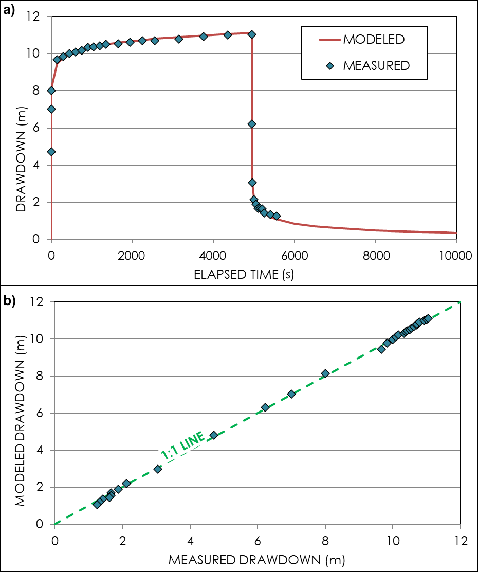
Figure 72 ‑ Example of a calibrated model results matching measured aquifer test results. a) measured drawdowns versus time (blue diamonds) compared to the final calibrated model results (red line); b) a direct comparison of individual modeled drawdowns to the corresponding measured drawdowns with comparison to a 1:1 line.
One challenge associated with calibrating groundwater models is that, in some cases, a variety of model configurations can match the available data equally well. When this happens, model predictions are not reliable. This issue can be alleviated by having a variety of field measurements to calibrate the model (i.e., not only water level measurements but also flow measurements). Exercise 19⮧ illustrates this problem using the model of Dupuit flow that was discussed in Section 6.3.2.
Evaluate and Quantify Uncertainty
As previously defined, a model is a simplified representation of a natural system. Aquifers are complex, heterogeneous systems that are extremely difficult to characterize and understand. In addition, aquifers are underground, and even when we have extensive networks of boreholes and related data, we are only directly observing a vanishingly small fraction of the overall volume of the aquifer. When hydrogeologists and engineers make groundwater flow models for predictions and forecasting, they generally make many simplifying assumptions about the input parameters—for example, assuming that the entire aquifer can be simulated with a single permeability—with very little verification of the validity of the final model results. To state it in another way, groundwater models always have various levels of uncertainty that range from the input parameters chosen to the final output and predictions.
Rather than develop models to simply make predictions with the hope that the input parameters are appropriate, models can be developed to evaluate and determine the level of predictive uncertainty associated with the available input parameters. This approach typically involves applying ranges of input parameters—for example, permeability—that are based on the ranges of available data, then using specialized software to develop large numbers of model simulations that are matched to available data associated with the predictions of interest—for example, drawdowns or water levels. The results of these models can be used to quantify the amount of risk associated with various management strategies—for example, installing a proposed well field—which can then be used to inform project managers and project investment.
A more detailed overview of model uncertainty analysis is beyond the scope of this book. Readers are encouraged to review the papers and other instructional materials at the Groundwater Modelling Decision Support Initiative (GDMSI) website at https://gmdsi.org/↗.