
11.6 Graphical Representations of Geochemical Data
Dealing with large amounts of geochemical data can be facilitated by using some standard graphical methods for displaying and analyzing the data. The following sections contain general descriptions of methods that are commonly used for presenting and interpreting groundwater chemistry data.
Piper Diagrams
Piper diagrams are a specific type of ternary diagram used to plot the concentrations of the major cations and anions (Figure 81). The Piper diagram consists of two ternary diagrams—one for cations and one for anions—and a central diamond‑shaped field into which the cation and anion values are projected. The relative percentages of the concentrations (in meq/L) of the three major cations (Ca, Mg, and Na) are plotted on the ternary diagram to the left. Usually, potassium and sodium are added together since they are similar in size and readily substitute for each other in minerals. The same is done with the three major anions (Cl, HCO3, and SO4). The location of each point is then projected up into the central area, and the intersection of the projections defines a point on the central field.
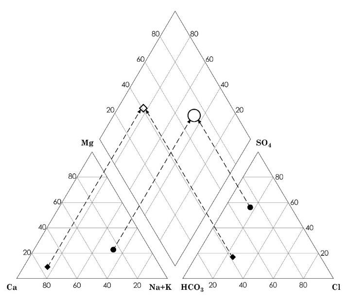
Figure 81 ‑ Piper diagram: the upper diamond integrates the ions from the bottom left triangle (cations) and lower right triangle (anions)
Piper diagrams are good for looking at lots of data, because they can show distinct groups of water types (Figure 82) as well as the relationships between those groups. Exercise 23⮧ provides an opportunity to plot the water analysis of Exercise 20 and 21 on a piper diagram.
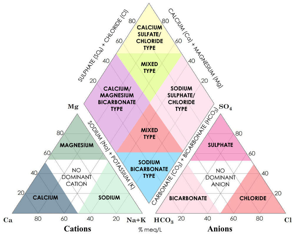
Figure 82 – Water types as delineated by the location of a water analysis on a Piper diagram (modified from Hatari Labs).
An example is given in Figure 83. The data are from groundwater samples taken from wells in Presidio County, Texas. Samples from wells in the Rio Grande Alluvium and from those in the upgradient volcanic formations fall into distinct fields on the diagram. The samples in the Presidio Basin sediments, located between the igneous uplands and the Rio Grande Alluvium, fall into a broad area that overlaps both fields with some samples clearly falling in the Igneous/Volcanic field, some in the Rio Grande Alluvium field, and some along the boundary. The locations of the Presidio Basin samples on the plot can therefore provide clues about the origins of the water in those wells.
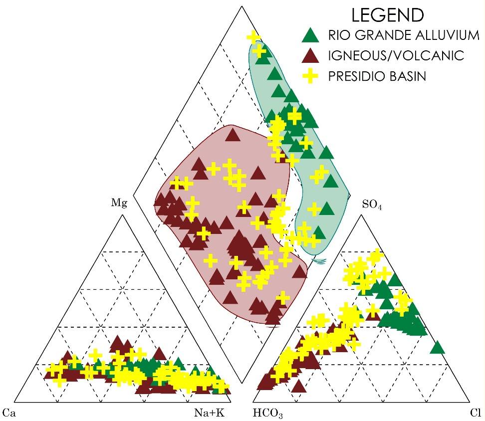
Figure 83 ‑ Piper diagram of analytical data from water samples taken in Presidio County, Texas (McKiernan and Uliana, 2005; all data acquired from the Texas Water Development Board Water Well Database in February 2005).
Stiff Diagrams
Stiff diagrams are a way of representing analyses from an individual water sample. A Stiff diagram is basically a graph that has concentration (in meq/L) on the horizontal axis and the major cations and anions on the vertical axis (Figure 84). The central vertical line represents zero concentration, and the cation concentrations are to the left while the anion concentrations are to the right. The concentrations are plotted, and the points are joined with a solid line to create a polygon. The utility of these diagrams is that their shape gives the viewer an instantaneous picture of the water chemistry. For example, Figure 84a is from a water sample that contains predominantly calcium and sulfate, while Figure 84b is from a water sample that is mostly sodium and chloride. We can use these diagrams to compare samples and to identify groups of samples.
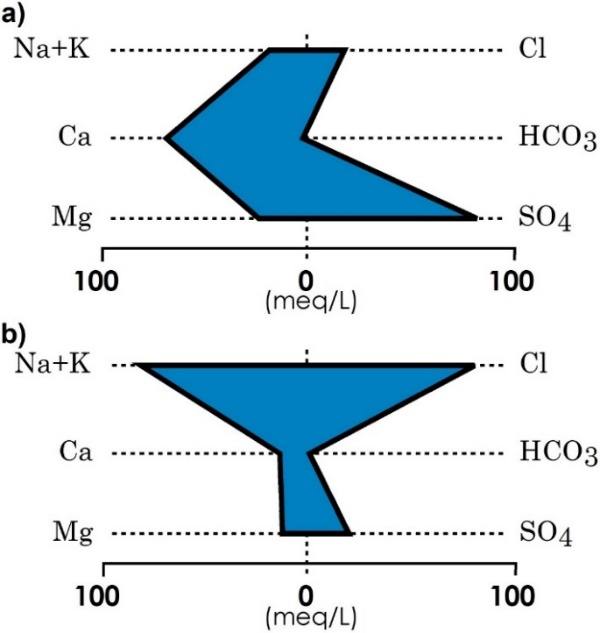
Figure 84 ‑ Stiff diagrams.
Case study: Using Geochemical Diagrams to Identify a Contamination Source
The following is an example of an application of Piper and Stiff diagrams in an area that was allegedly impacted by leaking deep salt-water disposal (SWD) injection wells (Uliana, 2005). Several shallow wells located on a ranch in West Texas (north of Orla, TX, USA) had suddenly become too salty for the cattle to tolerate. The well owners suspected that SWD injection wells located on the ranch property were responsible for the contamination. The SWD injection wells are injecting brines that contain high concentrations of sodium (Na+) and chloride (Cl‑). The SWD wells are extremely deep and the head in the injection intervals is much higher than ground surface so any breach in the casing or cement of the injection wells will result in brine moving into the shallow aquifer. Samples were taken from several of the shallow ranch wells in the vicinity of the brine injection wells and analyzed for the major cations and anions. Figure 85 shows the results of those samples, plotted as Stiff diagrams.
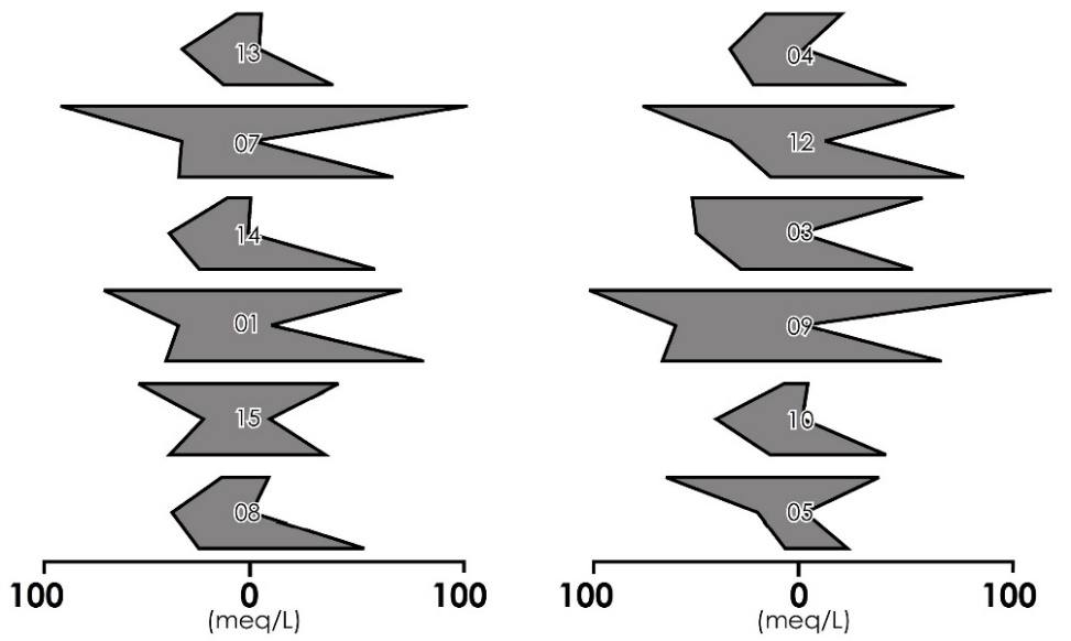
Figure 85 ‑ Stiff diagrams from shallow wells near brine disposal wells (modified from Uliana, 2005).
The TDS, sodium concentrations, chloride concentrations, and the shapes of the Stiff diagrams suggested that the samples fell into two distinct groups; a lower TDS group with a chemical signature that had more calcium and sulfate, and a higher TDS group that had more sodium and chloride (Figure 86). Groundwater samples taken from wells located away from the ranch indicate that the natural groundwater in this region is dominated by calcium and sulfate with very little sodium and chloride. It was therefore hypothesized, based on these data, that the Group 1 samples are more like the natural water chemistry with minimal impact from the brine injection wells, while the Group 2 samples have been impacted by saline water.
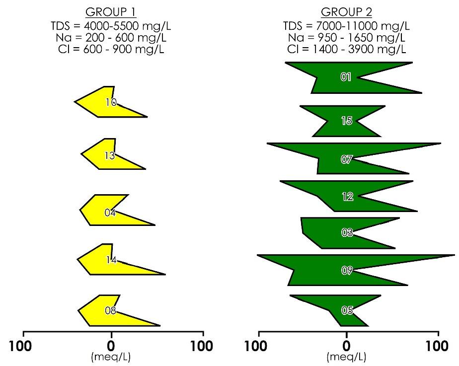
Figure 86 ‑ Samples are placed into groups based on concentration and shapes of the Stiff diagrams (modified from Uliana, 2005).
Plotting the same data on a piper diagram (Figure 87) supports the hypothesis that the brine injection wells could be responsible for the contamination. The background samples from off‑site wells plot in a restricted region that is dominated by calcium and sulfate, which is consistent with the abundance of gypsum and anhydrite in the local aquifer. The brine injection wells are high sodium and sulfate as expected, and they plot in a similarly restricted area. The wells in Group 1 plot very close to the background wells, while the Group 2 wells plot between the brine injection wells and the Group 1 wells. This is also consistent with the hypothesis.
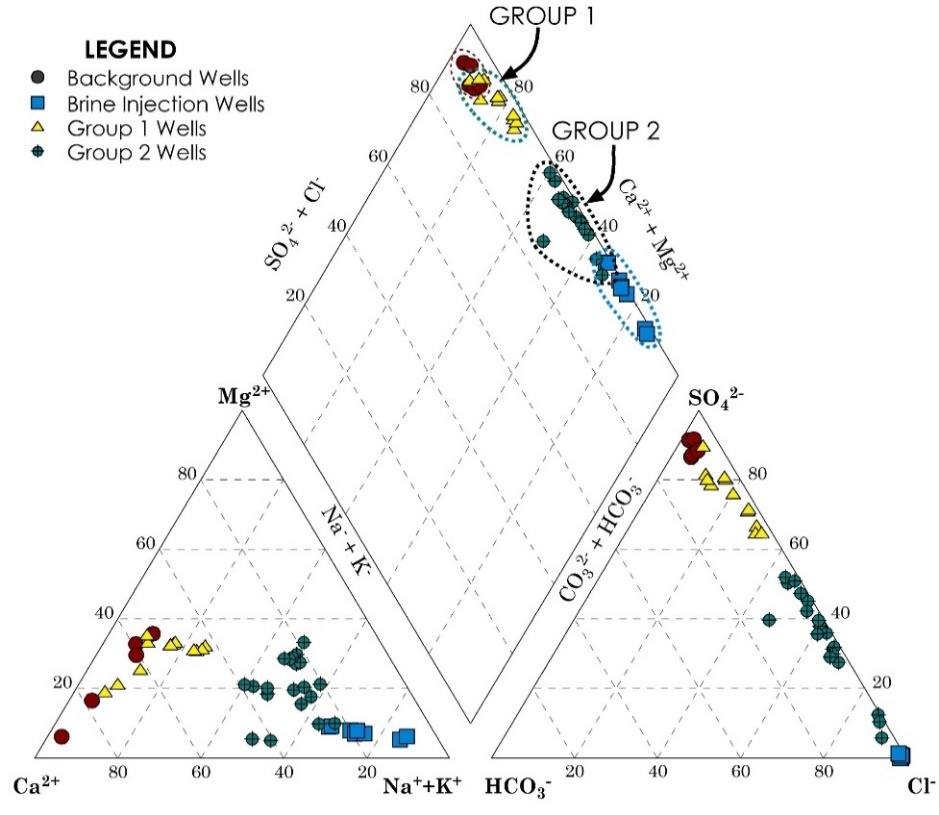
Figure 87 ‑ Piper diagram for water samples taken in Culberson County, Texas (modified from Uliana, 2005).
Plotting the Stiff diagrams on a map with their well locations (Figure 88) indicates a clear pattern with the Group 2 samples closest to the brine injection wells, while the others are farther away. This suggests that the Group 2 samples have been contaminated by the brine injection wells, and that the Group 1 samples reflect the natural water chemistry.
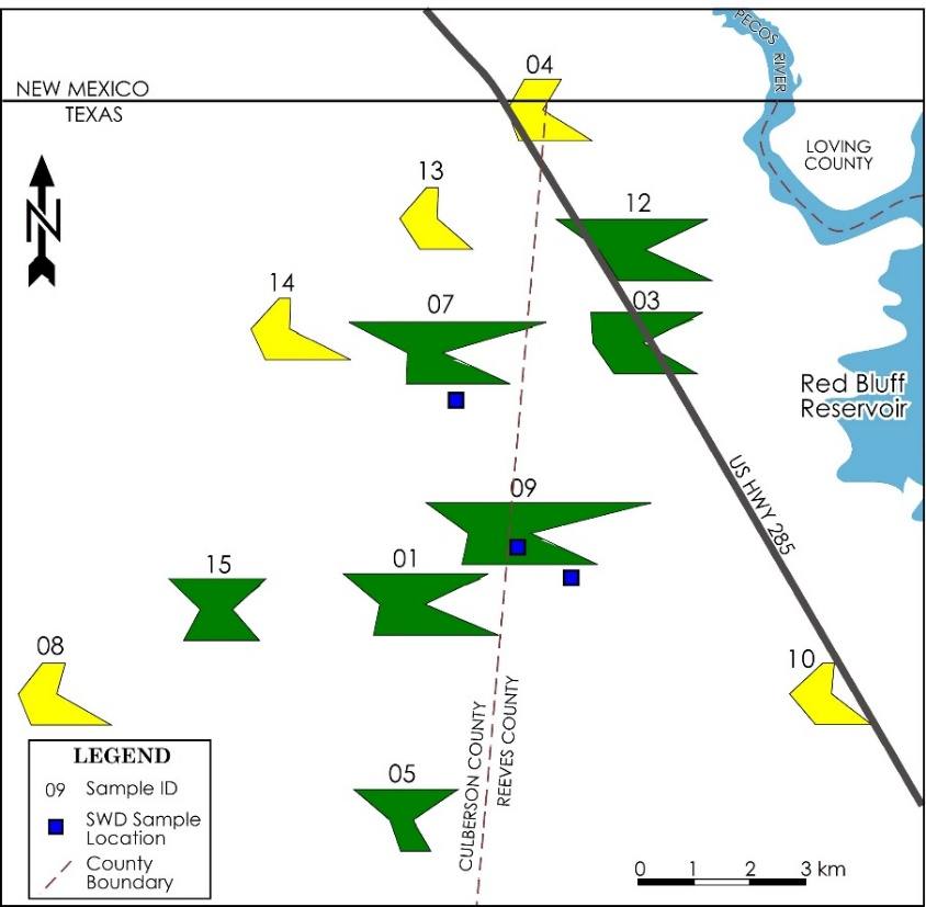
Figure 88 ‑ Map of sample locations with Stiff diagrams and location of brine injection wells (modified from Uliana, 2005).
Schoeller Diagrams
Schoeller diagrams are another graphical way of expressing the chemistry of a single sample (Figure 89). In these diagrams, the horizontal axis is each of the major cations and anions, while the vertical axis is the concentration of each in meq/L on a log scale. When the data are plotted, they are connected with straight‑line segments to create a crooked line that, like in the Stiff diagrams, gives an immediate picture of the chemistry of the samples that can then be compared to other samples.
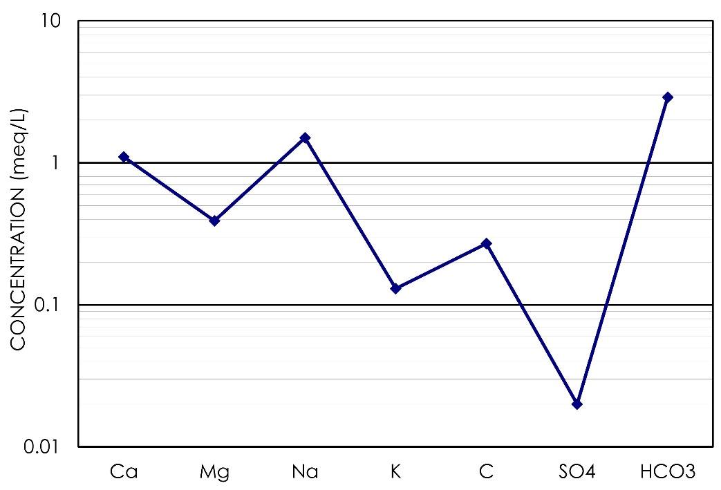
Figure 89 ‑ Schoeller diagram.