
16.3 Fracture Properties
Orientation
Fractures are three‑dimensional structures that are generally assumed to be planar or close to planar. Therefore, just like any planar structure we can characterize the orientation with strike and dip, where the strike is the line created by the intersection of the fracture with the horizontal plane, and the dip is the angle of the fracture plane below the horizontal plane. We can measure these orientations in the field or on aerial photographs, and then use rose diagrams (Figure 126), radial plots, or stereonets to present the distribution of these orientations.
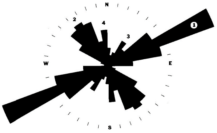
Figure 126 ‑ Sample bi‑directional rose diagram showing the strike direction of fracture sets in a rock formation with the length of the rose petal representing one of a variety of features such as the frequency of fractures in that set relative to all fractures in the rock, the length of the fractures in that set, the average magnitude of their dip. The numbered labels represent the 4 main fracture set directions.
Rose diagrams can be plotted on maps to show fracture trends and changes in orientation throughout a region. These diagrams can identify sets of fractures, which can then be related to groundwater flow directions using several methods, such as geochemical tracers.
Aperture
Fracture aperture is the distance between the fracture walls (Figure 127).
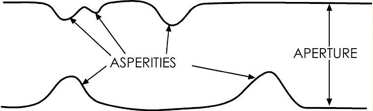
Figure 127 ‑ Fracture aperture and asperities on fracture wall.
In an idealized fracture with smooth walls and a constant aperture—that is, the fracture walls are parallel to each other—the hydraulic conductivity and the discharge are proportional to the aperture. However, rock fractures always have asperities that stick out from the wall of the fracture. These affect the properties of the fracture in the following ways.
- Asperities create roughness on the fracture surface. This roughness has several effects.
- Channelization of fluid along the surface of the fracture—most of the water flow only within channels on the fracture surface and not uniformly over its entire surface (Figure 128).
- Tortuosity (𝜏)—defined as the distance water travels divided by the straight‑line distance between two points, the more numerous the asperities and the larger their amplitude, the more tortuous the flow path, thus water must travel farther —this is sometimes defined as the reciprocal (Figure 129).
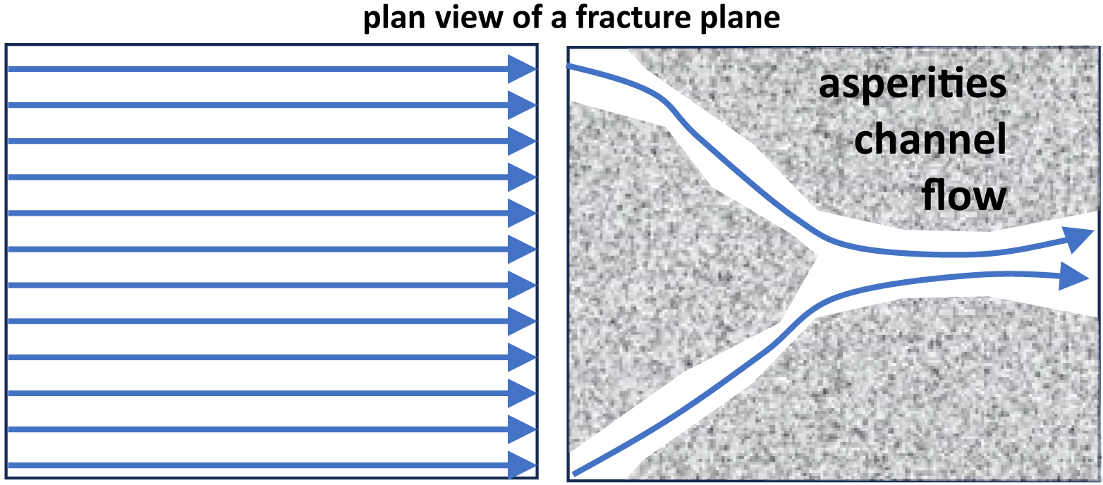
Figure 128 ‑ Plan view of a fracture surface: a) without asperities; and b) with channeling of flow along the surface of a fracture around asperities.
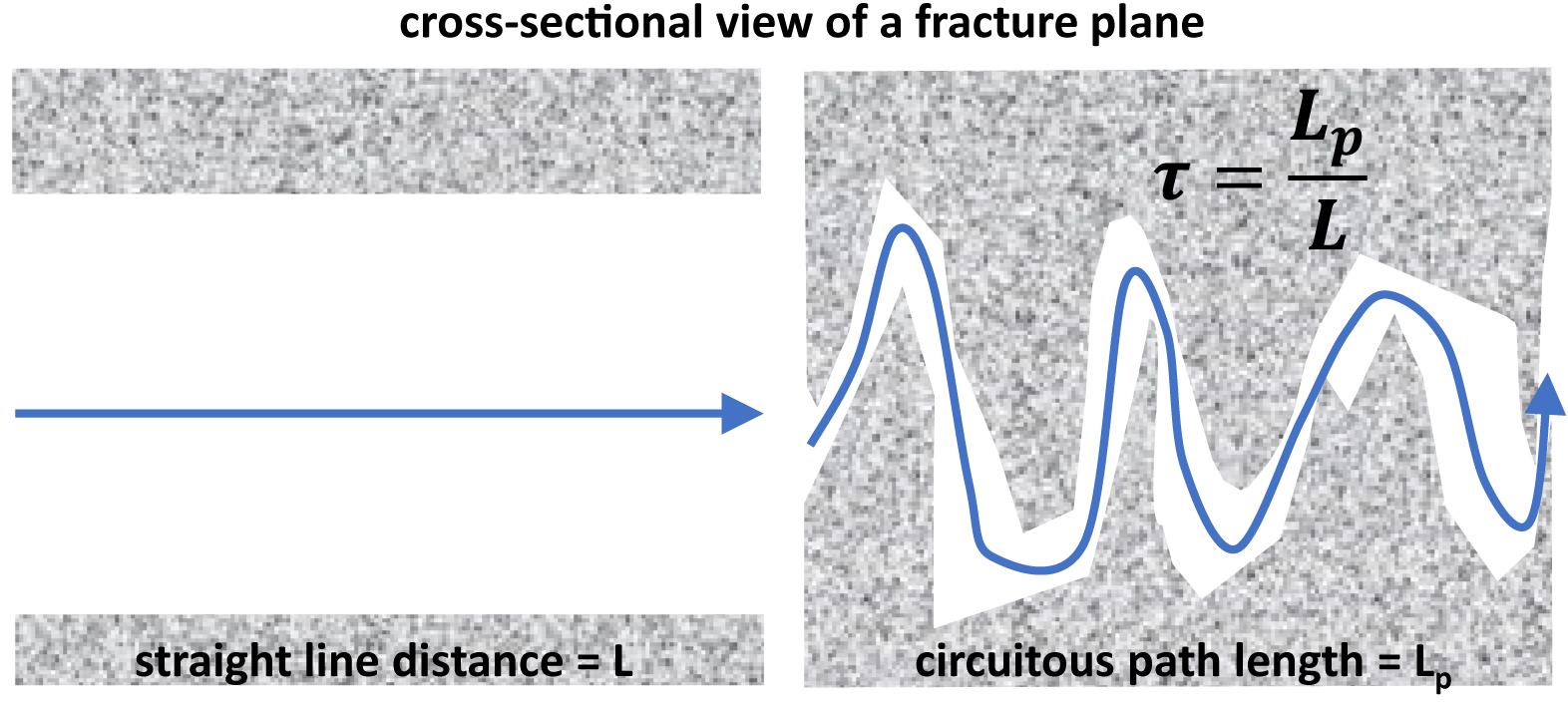
Figure 129 ‑ Cross sectional view of a fracture plane a) without asperities; and b) with asperities causing tortuous flow along the fracture.
- Friction associated with surface roughness impedes the flow of fluids. Friction also affects the geotechnical properties of the fracture—higher roughness means that the fracture is less likely to fail or activate in response to changes in stress.
- In the subsurface, where the fracture is under compressive stress, the asperities hold the fracture open.
Length, Width, and Depth
Fractures are three‑dimensional structures that, in addition to aperture, have a length and a width. An idealized fracture in the subsurface, which does not intersect the surface, will generally have an irregular elliptical shape with an aperture that is maximum near the middle and tapers off to the edges (Figure 130).
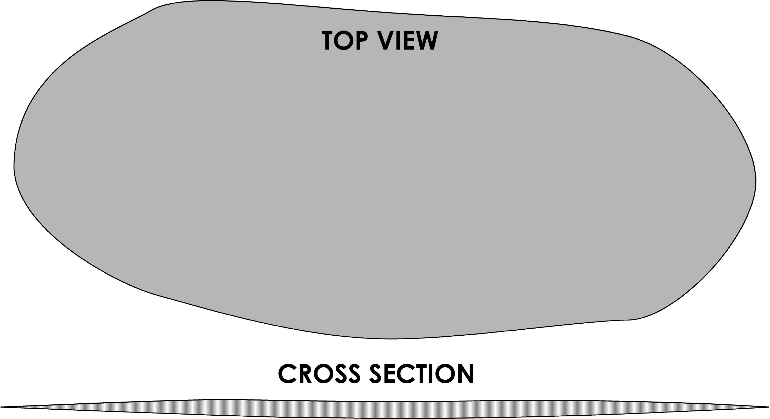
Figure 130 ‑ General fracture geometry.
When we talk about length and width, we are generally talking about the dimension that is exposed at the Earth’s surface—either at an outcrop or identified from an aerial photo. In outcrop, we frequently cannot see the ends of the fracture—it either terminates at the top of the outcrop or it terminates somewhere underground, or both. Length is generally used to describe the exposed length of a vertical fracture in an outcrop; width is often used to describe horizontal fractures. Depth refers to the distance that the fracture goes into the outcrop. This can sometimes be measured or observed using geophysical methods—ground penetrating radar, shallow seismic, electromagnetic—or using boring logs. However, geophysical methods are limited because they do not quantify whether the fracture is open (i.e., able to support flow) or filled and sealed.
Spacing and Density
A given volume of rock will generally not have only a single fracture in it; rather, there will be several fractures, and some of those fractures will have similar orientations due to the fact that they were formed by the same stresses. The spacing of the fractures refers to the distance from one fracture to the next; the density of fractures refers to the number of fractures in a unit volume of rock.
- Spacing is measured by running a scanline or traverse across an exposed rock face and measuring the distance between the points where the fractures intersect the scanline.
- Density is measured by adding up the lengths of all the fractures in a volume or area of rock and dividing the total length by the volume, or area. We frequently use area because these studies are often two‑dimensional outcrop studies—that is, on the surface—rather than three‑dimensional subsurface studies.
Spacing and density seem to be related to the aperture. Studies have indicated that, in specific rocks, there are direct relationships between fracture spacing and aperture—that is, smaller apertures tend to be more closely spaced, and vice versa. This relationship seems to hold across several scales—from thin section to outcrop to air photo—and if it holds true it could have a major impact on the way we model fractured systems.
Connectivity
Fractures are only effective as conduits for fluid flow if they are connected to each other. This is especially true in purely fractured or fractured formation systems. Fracture connectivity can be evaluated by observing fracture terminations and plotting the results on ternary diagrams. There are four basic types of fracture terminations (Figure 131a).
- Abutting (A)—the fracture ends in the middle of another fracture.
- Blind (B)—the fracture ends in the middle of the rock.
- Crossing (C)—the fracture crosses another fracture.
- Diffuse (D)—the fracture ends in a diffuse set of smaller fractures.
The number of each type of fracture termination can be counted in outcrop and plotted on a ternary diagram. Since there are four categories, and only three endmembers on a ternary diagram, two of the categories must be grouped. There are two different ways of plotting; the Barton and Hsieh (1989) method (Figure 131b) and the Laubach (1992) method (Figure 131c). In the Barton and Hsieh method, blind and diffuse terminations are lumped together. In the Laubach method, the abutting and crossing terminations are lumped together as connected. Exercise 27⮧ demonstrates one way that ternary diagrams of fracture termination can be applied.
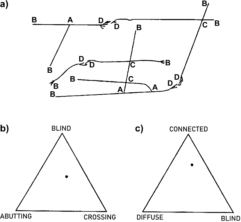
Figure 131 ‑ Fracture terminations. a) Type of termination: A=abutting; B=blind; C=crossing; D=diffuse (from Laubach, 1992). Ternary diagrams for displaying the number of different fracture types: b) as proposed by Barton and Hsieh (1989); and c) as proposed by Laubach (1992).