
7.2 Steady‑State Conditions in an Unconfined Aquifer
The mathematics for steady‑state flow in an unconfined aquifer are based on Darcy’s Law and the conservation of mass. Under steady‑state conditions the gradient within the cone of depression does not change over time and the discharge at any radial distance (within the cone of depression) from the pumping well is equal to the hydraulic conductivity (K) times the cross‑sectional area (2πrh), times the gradient (‑dh/dr) at that radial distance. In the case of the unconfined system, the head values (h) are defined as the difference between the water table elevation and the elevation of the aquifer base (Figure 20).
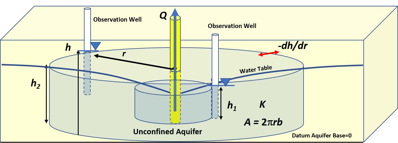
Figure 20 – The radial flow of water through a cylindrical area within the steady‑state cone of depression created in an isotropic and homogeneous unconfined groundwater system when pumping a well at a constant rate. The well discharge (Q) passes through a cross sectional area (A=2πrh), of a material that has a hydraulic conductivity (K) under a gradient (‑dh/dr) directing water to the well. The head (h) is equal to the saturated thickness measured as the water table elevation minus the elevation of the base of the unconfined system.
To formulate an analytical solution, the Thiem (1906) general assumptions are applied along with the Dupuit (1863) assumptions that the slope of the water table is equal to the hydraulic gradient and flow is horizontal (e.g., Fetter 2001; Kruseman & de Ritter, 2000). The resulting equation describes steady‑state flow in an unconfined system as shown in Equation (18).
| [latex]Q = - (2\pi rh)K\left( \frac{dh}{dr} \right)[/latex] | (18) |
|---|
where:
| Q | = | constant discharge (L3T‑1) |
|---|---|---|
| r | = | radial distance to the pumping well (L) |
| h | = | saturated thickness of the aquifer measured from the aquifer base (L) |
| dh/dr | = | hydraulic gradient (dimensionless) |
An analytical solution is derived by integration with the head in the unconfined unit defined as the height of saturation above the unconfined aquifer base, h1. The closer observation well is defined by values of r1 and h1, and the farther observation well represented by values r2 and h2 (Figure 21).
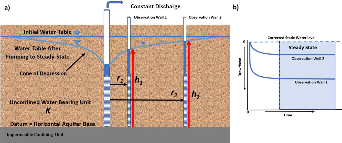
Figure 21 – Cross section of an unconfined groundwater system under steady‑state conditions. a) Location of observation wells and parameters required by the Thiem equation. The saturated thickness (h) at an observation well is measured from the horizontal base of the system. b) Drawdown time curves for the observation wells. The dashed vertical line and light blue shading indicate when drawdown reaches and remains at steady state.
The resulting analytical solution is given as Equation (19).
| [latex]K = \frac{Q}{\pi\left( h_{2}^{2} - h_{1}^{2} \right)}\ln\left( \frac{r_{2}}{r_{1}} \right)[/latex] | (19) |
|---|
where:
| K | = | unconfined unit hydraulic conductivity (LT‑1) |
|---|---|---|
| Q | = | constant pumping rate (L3T‑1) |
| h2 | = | saturated thickness at well 2 furthest from the pumping well (L) |
| h1 | = | saturated thickness at well 1 furthest from the pumping well (L) |
| r2 | = | radial distance to observation well 2 (L) |
| r1 | = | radial distance to observation well 1 (L) |
The use of this equation assumes that once heads have reached steady state the change in saturated thickness at observation locations are small—less than 2 to 10 percent, depending on the literature reference.
Example
Assume a well is pumping in an unconfined aquifer at 1,500 m3/d. The original saturated thickness is 30 m. After reaching steady state the saturated thickness at observation Well 1 located 37 m from the pumping well is 26.9 m. The steady state saturated thickness at observation well 2, located 147 m from the pumping well, is 29.2 m. The hydraulic conductivity can be estimated for the unconfined system using Equation (19).
[latex]K = \frac{1,500\ \frac{m^{3}}{d}}{3.14\ \left( ({29.2m)}^{2} - ({26.9m)}^{2} \right)}\ln\left( \frac{147\ m}{37\ m} \right) = \ 5.11\ \frac{m}{d}[/latex]
As with the confined aquifer equation, the saturated thickness of the aquifer at any radial distance from the pumping well can be computed if the aquifer hydraulic conductivity, well discharge, and the saturated thickness at a radial distance at one observation well are known.
Again, when applying the Thiem equation for unconfined aquifers it is assumed that the head at observation wells is measured from the horizontal base of the aquifer so that it corresponds to the saturated thickness. The values of total head are not used in this equation as they are in the Thiem equation for confined groundwater systems. A common mistake is to use head values based on a datum other than the aquifer base (e.g., mean sea level). This will result in large errors in the estimated value of K.
Jacob (1963) proposed a modification of the Thiem equation for use with a water table system where drawdown becomes significant (i.e., 10 to 25 percent of the initial saturated thickness) at observation wells during testing (Figure 22). His method adjusted the observed drawdown (not saturated thickness), s1 and s2, to values that would occur if no significant dewatering took place (less than 2 to 10 percent depending on the reference source: Jacob, 1950; United States Department of the Interior (USDI), 1981) as shown in Figure 22. Calculations of K and T are then computed using the Thiem representation.
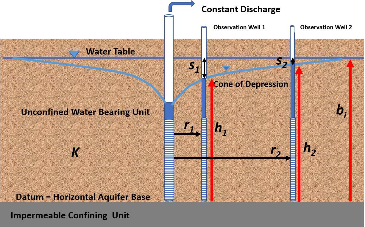
Figure 22 – The Jacob (1963) approach to estimating T for the steady‑state pumping of an unconfined aquifer with significant drawdown. The drawdown at the two observation wells is s1 and s2, respectively. The pre‑pumping saturated thickness is represented by bi. The saturated thickness at the observation wells is h1 and h2, respectively.
Lohman (1972) presents the unconfined formulation in terms of corrected drawdown as shown in Equations (20) and (21) for K and T respectively. The log base 10 is used in Lohman’s equations so it is useful to know that ln(x)=2.3log(x).
| [latex]K = \frac{- Q\ 2.3\ \log\left( \ \frac{r_{2}}{r_{1}} \right)}{\frac{2\pi b_{i}\ \left( \left( b_{i}^{2} - 2b_{i}s_{2} + s_{2}^{2} \right) - \left( b_{i}^{2} - 2b_{i}s_{1} + s_{1}^{2} \right) \right)}{2b_{i}}}[/latex] | (20) | |
|---|---|---|
| [latex]T = \frac{- Q\ 2.3\ \log\left( \ \frac{r_{2}}{r_{1}} \right)}{2\pi\ \left( \left( s_{1} - \frac{s_{1}^{2}}{2b_{i}} \right) - \left( s_{2} - \frac{s_{2}^{2}}{2b_{i}} \right) \right)}[/latex] | (21) |
where:
| bi | = | initial (pre‑pumping) unconfined saturated thickness (L) |
|---|---|---|
| K | = | hydraulic conductivity (LT‑1) |
| Q | = | constant discharge rate (L3T‑1) |
| r2 | = | radial distance to observation well 2 (L) |
| r1 | = | radial distance to observation well 1 (closest) (L) |
| s1 | = | drawdown at observation well 1 (closest) (L) |
| s2 | = | drawdown at observation well 2 (L) |
| T | = | transmissivity (L2T‑1) |
Using Equation (21) the drawdown correction is equal to s2/2b. If the magnitude of the correction is small, the computed T value will not change much. The correction is recommended when the pre‑pumping saturated thickness is affected by 10 to 25 percent at the measuring point (Kasenow, 2001; USDI, 1981). Kasenow (1995, 1997) developed additional approaches to correct observed drawdown data when reductions exceed 25 percent.
Example of Graphical Method
Steady‑state analyses require information from a pumping test that includes the measured drawdown (corrected‑static head ‑ pumping head) at two locations (i.e., two different radial distances from the pumping well). Lohman (1972) presents a graphical distance‑drawdown method using corrected drawdown to solve for T under confined and unconfined conditions. A graphical semi‑log, distance‑drawdown graph is shown in Figure 23. To represent confined aquifers, Equation (21) is simplified by representing the change in drawdown with distance with the change in drawdown over one log cycle of radial distance (i.e., ∆slog‑r/(∆log(r))) to obtain Equation (22). ∆slog‑r is purposefully selected as the drawdown change over one log cycle of distance so that ∆slog‑r/(∆log(r)) becomes ∆slog‑r divided by 1 (e.g., ∆(log r) = log 100 ‑ log 10 = 1).
| [latex]T = \frac{2.3\ Q}{\frac{2\pi{\mathrm{\Delta}s}_{log - r}}{\mathrm{\Delta}\ (\log\ r)}}[/latex] | (22) |
|---|
where:
| T | = | transmissivity (L2T‑1) |
|---|---|---|
| Q | = | constant discharge (L3T‑1) |
| ∆slog‑r | = | change in drawdown over one log cycle of distance (positive) (L) |
| ∆ (log r) | = | difference in log of radial distances that differ by one order of magnitude (dimensionless) |
When drawdowns need correction for unconfined aquifer dewatering then Equation (23) is used.
| [latex]T = \frac{2.30\ Q}{\frac{2\pi\mathrm{\Delta}\left( s - \frac{s^{2}}{2b_{i}} \right)}{\mathrm{\Delta}\ \log\ r}}[/latex] | (23) |
|---|
where:
| T | = | transmissivity (L2T‑1) |
|---|---|---|
| Q | = | constant discharge (L3T‑1) |
| ∆(s‑(s2/(2bi)) | = | change in corrected drawdown over one log cycle of distance (positive) (L) |
| ∆ log r | = | one log cycle of radial distance (dimensionless) |
| bi | = | initial (pre‑pumping) unconfined saturated thickness (L) |
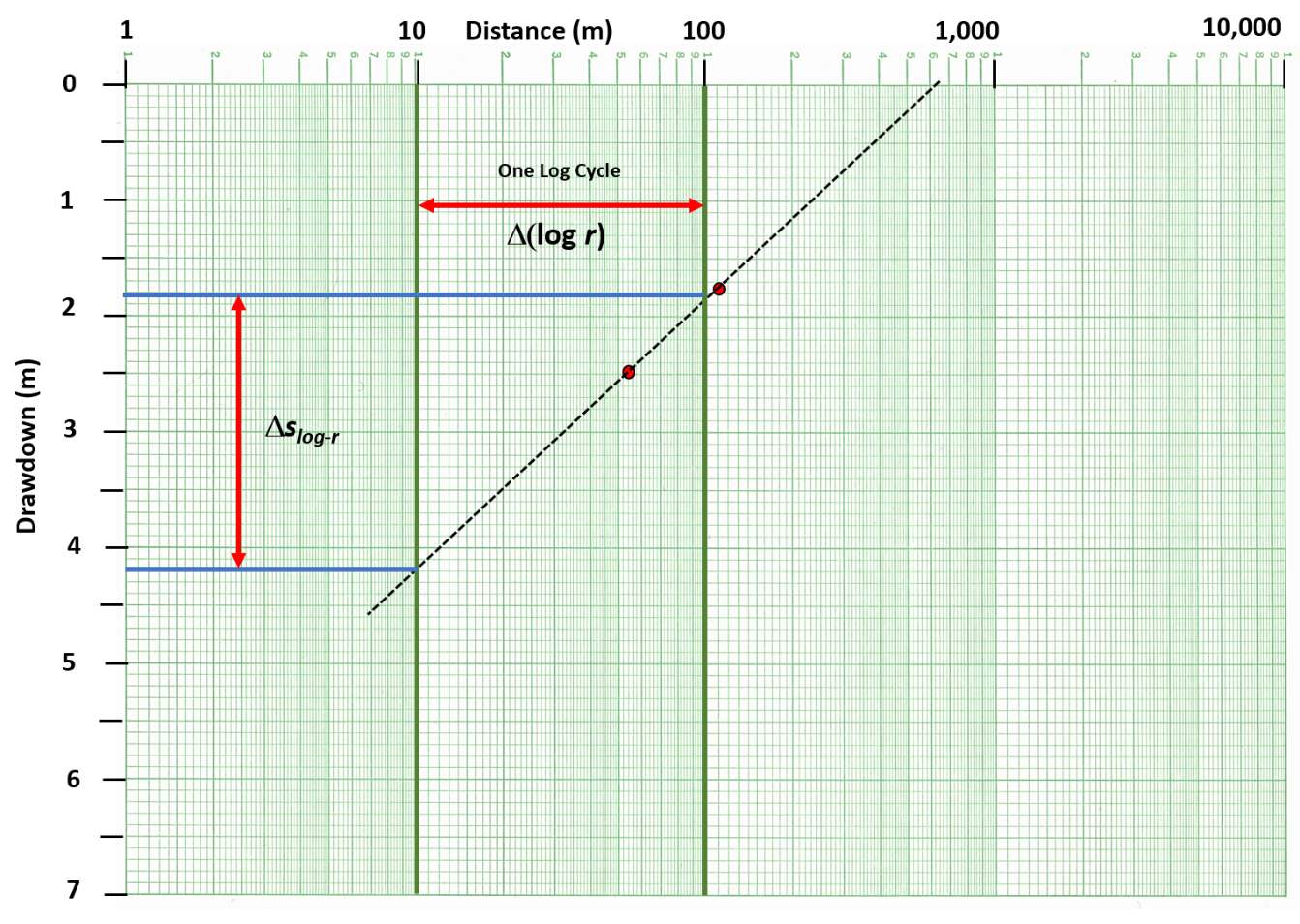
Figure 23 – Plot of the drawdown at two observation wells (red dots) after steady‑state conditions were reached during a constant discharge test of a confined aquifer. The slope of the line is defined over one log cycle as ∆slog‑r/∆(log r) (red double arrows). ∆slog‑r/∆(log r) is equal to 2.4 m / 1.
Example
The distance‑drawdown plot presented in Figure 23 is the steady‑state drawdown observed at observation wells located 55 m and 123 m from a production well pumping at a constant rate of 1,400 m3/d. The wells fully penetrate a 24 m‑thick confined sand. From the graph, ∆slog‑r = 2.4 m. T is computed using Equation (22).
[latex]T\ = \ \frac{2.3\ 1,400\frac{m^{3}}{d}}{\frac{2\ (3.14)\ (4.2\ m\ - \ 1.8\ m)}{1}} = \ 214\frac{m^{2}}{d}[/latex]
Sections 8 through 11 address the development and application of simplified analytical models that represent how groundwater systems respond to pumping and how T and S are estimated under transient conditions.