
Box 11 AQTESOLV Solutions to Exercises
This box provides solutions to Exercises 2, 3, 5, and 7 using a standard version of AQTESOLV. The manual curve match and user fitted lines to semi‑log analyses presented in Section 21 “Exercise Solutions” are compared with the results for the same problems generated using AQTESOLV. Once again, the three leading software developers provide free demonstration or trial versions.
- AQTESLOV (aqtesolv.com↗)
- AquiferTest (waterloohydrogeologic.com/download-trial/↗)
- Aquiferwin32 (zip file that will download when this link is clicked↗)
These programs can be used to solve most, if not all, of the pumping test and slug test Exercises 2, 3, 5, and 7.
In many agencies and businesses hydraulic test analyses are commonly completed using one or more of the three software packages discussed in this book (Section 13, Section 14.6, and Boxes 5, 6, and 7). The material presented in this box shows how the results of manual curve matching methods compare to analyses accomplished using AQTESOLV, as they are in the other two commercially available programs. When analyses of hydraulic test data sets are routinely required, it is suggested that one of the commercially available programs become part of your hydrogeologic toolbox.
Box 11.1 AQTESOLV Solution for Exercise 2
The manual solution for Exercise 2 involves matching field data to Theis type curves as delineated in Section 21. This box provides images of the Exercise 2 solutions for part a, c, and d, using AQTESOLV, followed by a table comparing the manual and AQTESOLV results.
The AQTESOLV image of match to the Theis solution for Observation well 1 at r = 66 m is shown in Figure Box 11‑1.
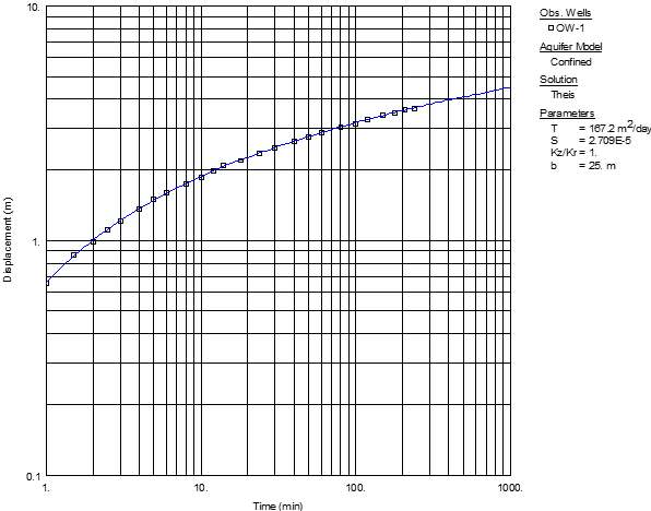
Figure Box 11‑1 AQTESOLV Theis solution for OW1 r = 66 m.
The AQTESOLV image of match to the Theis solution for Observation well 2 at r = 122 m is shown in Figure Box 11‑2.
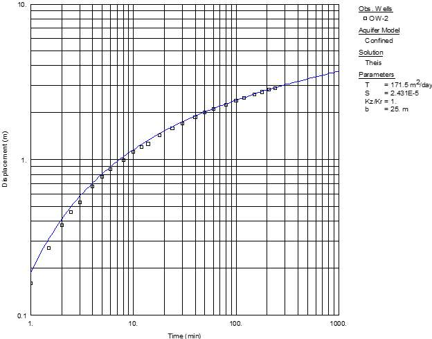
Figure Box 11‑2 AQTESOLV Theis solution for OW2 r = 122 m.
The AQTESOLV image of match to the Theis solution for Observation well 3 at r = 244 m is shown in Figure Box 11‑3.
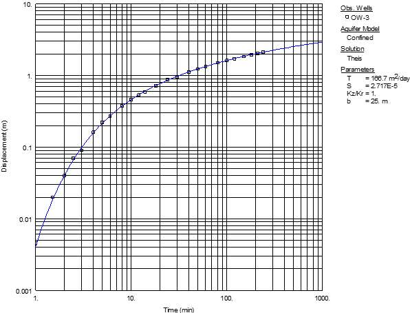
Figure Box 11‑3 AQTESOLV Theis solution for OW3 r = 244 m.
The AQTESOLV image for match to Cooper‑Jacob solution for Observation well 2 at r = 122 m is shown in Figure Box 11‑4.
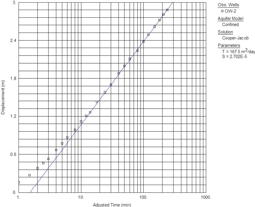
Figure Box 11‑4 AQTESOLV Cooper‑Jacob solution for OW2 r = 122 m.
The AQTESOLV image for a distance‑drawdown solution at 100 minutes is shown in 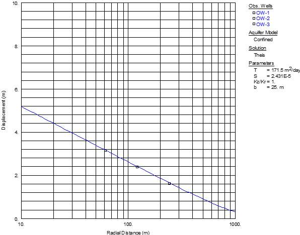
Figure Box 11‑5 AQTESOLV confined distance‑drawdown solution using OW1 r = 66 m., OW2 r = 122 m, OW3 r = 244 m at 100 minutes.
The results obtained by manual and automated fitting are compared in Table Box 11‑1.
Table Box 11‑1 ‑ Comparison between results in Solution Exercise 2 of Section 21 accomplished with hand‑fitted curve matching and AQTESOLV results.
| Manual | Automated | |||
|---|---|---|---|---|
| T m2d‑1 | S | T m2d‑1 | S | |
| Exercise 2 | ||||
| Exercise 2a r = 66 m | 165 | 3×10‑5 | 167 | 2.7×10‑5 |
| Exercise 2a r = 122 m | 159 | 3×10‑5 | 172 | 2.4×10‑5 |
| Exercise 2a r = 244 m | 165 | 2×10‑5 | 167 | 2.7×10‑5 |
| Exercise 2c r = 122 m | 164 | 6×10‑6 | 168 | 2.7×10‑5 |
| Exercise 2d | 163 | 3×10‑5 | 172 | 2.4×10‑5 |
Box 11.2 AQTESOLV Solution for Exercise 3 a and b
The manual solution for Exercise 3 involves matching field data to Hantush‑Cooper leaky aquifer type curves as delineated in Section 21. This box provides images of the Exercise 3 solution using AQTESOLV, followed by a table comparing the manual and AQTESOLV results.
The AQTESOLV image of the Hantush‑Cooper leaky aquifer solution match to the field data Figure Box 11‑6.
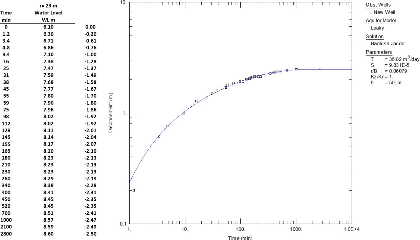
Figure Box 11‑6 ‑ AQTESOLV Hantush‑Jacob solution for observation well data. Parameters calculated from the fit are shown in the upper right. Drawdown data computed and shown on left hand side of diagram.
Noting the discrepancy between the manual and automated results and knowing that it was difficult to read the r/B value for the manual solution, AQTESOLV was used to generate type curves for r/B from 0.02 to 3 and overlay the data on those curves as shown in Figure Box 11‑7. This made it much easier to determine the r/B value.
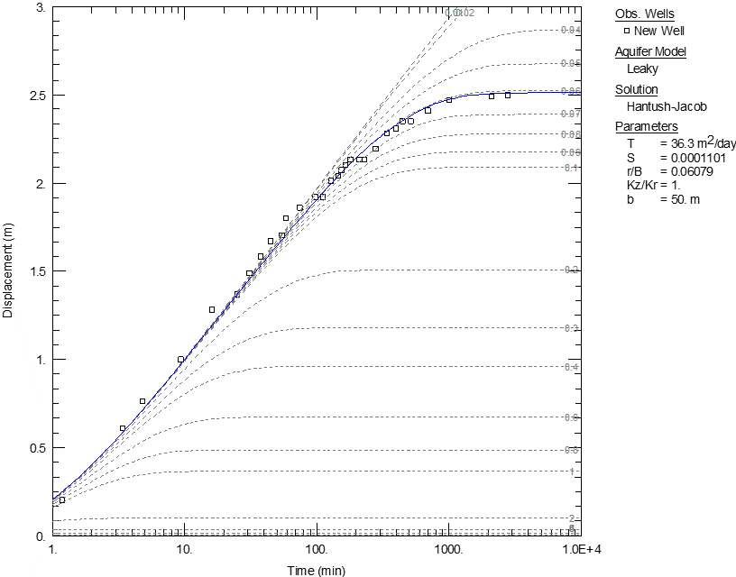
Figure Box 11‑7 ‑ AQTESOLV Hantush‑Jacob solution for observation well data. In AQTESOLV an option to compute and show additional type curves for the chosen analysis method is available. Here values of r/B between 0.02 and 3 were generated from the analytical solution. The automated curve matched r/B value of 0.06069 is shown on this family of curves.
The results obtained by manual and automated fitting are compared in Table Box 11‑2.
Table Box 11‑2 ‑ Comparison between results in Solution Exercise 3 of Section 21 accomplished with hand‑fitted curve matching and AQTESOLV results.
| Manual | Automated | |||||
|---|---|---|---|---|---|---|
| Exercise 3 | T m2/d | S | K’ m/d | T m2/d | S | K’ m/d |
| OW = 23 m | 32.5 | 1.2 x 10‑4
≈ 1 x 10‑4 |
0.0066 | 36.8 | 9.8 x 10‑5
≈ 1.0 x 10‑4 |
0.008* |
*Computed outside of AQTESOLV using r/B =0.06) as shown here.
[latex]K' = \frac{Tb'\left( \frac{r}{B} \right)^{2\ }}{r^{2}} = \frac{36.8\ \frac{m^{2}}{d}(30\ m)(0.06)^{2\ }}{{(23\ m)}^{2}} = 0.008\frac{m}{d}[/latex]
The Hantush‑Jacob visual curve matching and AQTESOLV results are similar. The application of either approach yields reasonable hydrogeologic values for this leaky confined aquifer data set.
Box 11.3 AQTESOLV Solution for Exercise 5
The manual solution for Exercise 5 involves analyzing a step drawdown test as delineated in Section 12. This box provides images of the Exercise 5 solution using AQTESOLV, followed by a table comparing the manual and AQTESOLV results. The AQTESOLV image of the analysis of the field data is presented in Figure Box 11‑8.
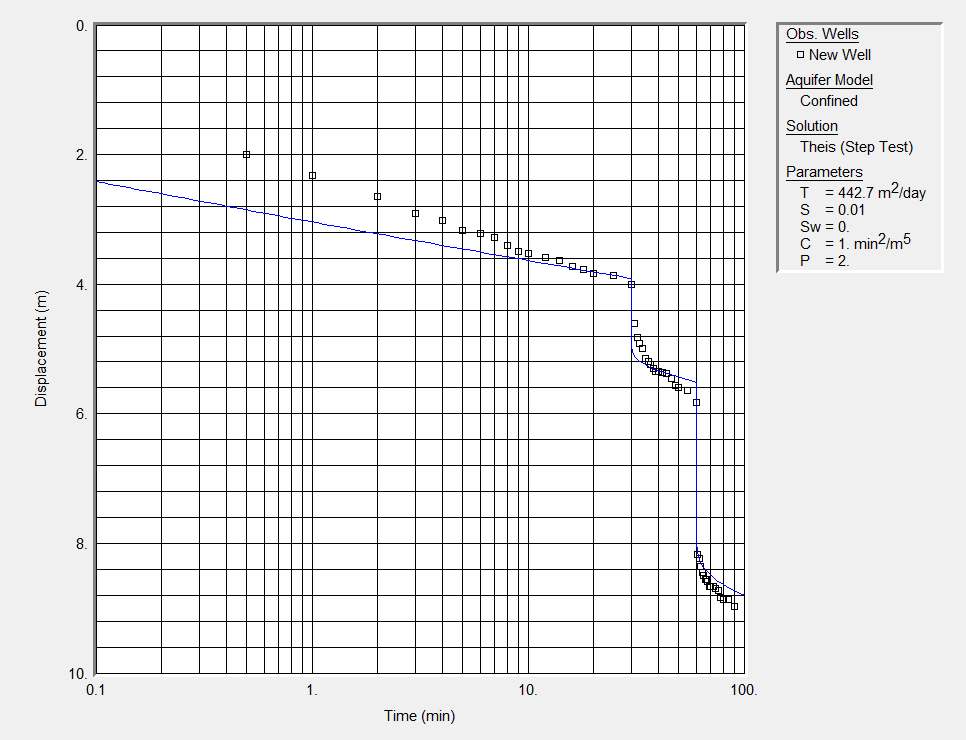
Figure Box 11‑8 AQTESOLV Theis solution variable pumping rate slug test analyses for a step drawdown test.
The results obtained by manual and automated fitting are compared in Table Box 11‑3.
Table Box 11‑3 ‑ Comparison between results in Solution Exercise 5 of Section 21 accomplished with manual analysis and AQTESOLV results.
| Manual | Automated | |||
|---|---|---|---|---|
| Exercise 5 | T m2/d | C d2/m5 | T m2/d | C d2/m5 |
| 214 | 3.0×10‑7 | 443 | 4.8×10‑7 * | |
*conversion: (1.0 min2/m5) (1 d / 1440 min)2 = 4.8 x10‑7 d2/m5
The T value obtained using AQTESOLV is higher than that obtained using manual methods. The values of C are similar. Generally, in this case inputting the step drawdown data and letting AQTESOLV generate an estimate of C, P, S, and T yielded poor estimates. In order to obtain values of C similar to the manual solution of Exercise 5, the range of parameter values were constrained including setting P (exponent of C) to 2 and limiting the maximum S value to 0.01. The generated S value is unreasonably high for a confined aquifer, however, constraining S to smaller values degraded the quality of fit to the data. In this case, careful analyses of model results are required to obtain reasonable values. It is recommended that manual analysis of step test data sets be performed before automated fitting. The manual analysis results serve as a check of the fitting program results.
Box 11.4 AQTESOLV Solution for Exercise 7
The manual solution for Exercise 7 involves analyzing a slug test as delineated in Section 14. This box provides images of the Exercise 7 solution using AQTESOLV, followed by a table comparing the manual and AQTESOLV results. The AQTESOLV image of the analysis of the field data is presented in Figure Box 11‑9.
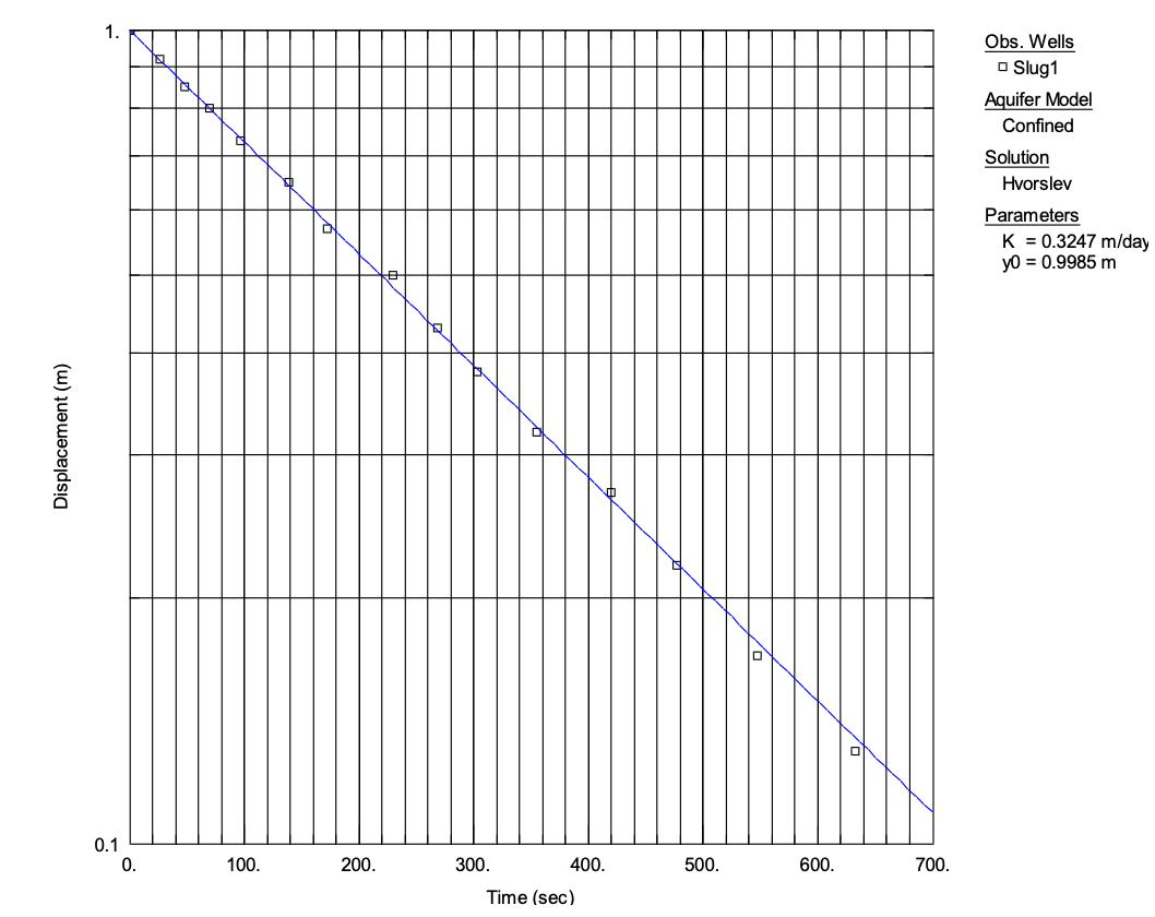
Figure Box 11‑9 AQTESOLV slug test analysis .
The results obtained by manual and automated analysis are compared in Table Box 11‑4.
Table Box 11‑4 ‑ Comparison between results in Solution Exercise 5 of Section 21 accomplished with manual analysis and AQTESOLV results.
| Manual | Automated | |
|---|---|---|
| Exercise 7 | K m/d | K m/d |
| using Equation (107) | 0.33 | 0.32 |
| using Equation (108) | 0.33 |
The Hvorslev hand fitted curve matching and AQTESOLV results are very similar. The application of either approach yields reasonable hydrogeologic values for this unconfined slug test data set.