
Solution Exercise 4
A well (A) pumping at 900 m3/d is located near a river as shown in the image below. The river penetrates a fractured, permeable, confined limestone. A second production well (B) is located 200 m from the first well. A previous pumping test of the formation at well A yielded a T of 75 m2/d and an S of 0.00003.
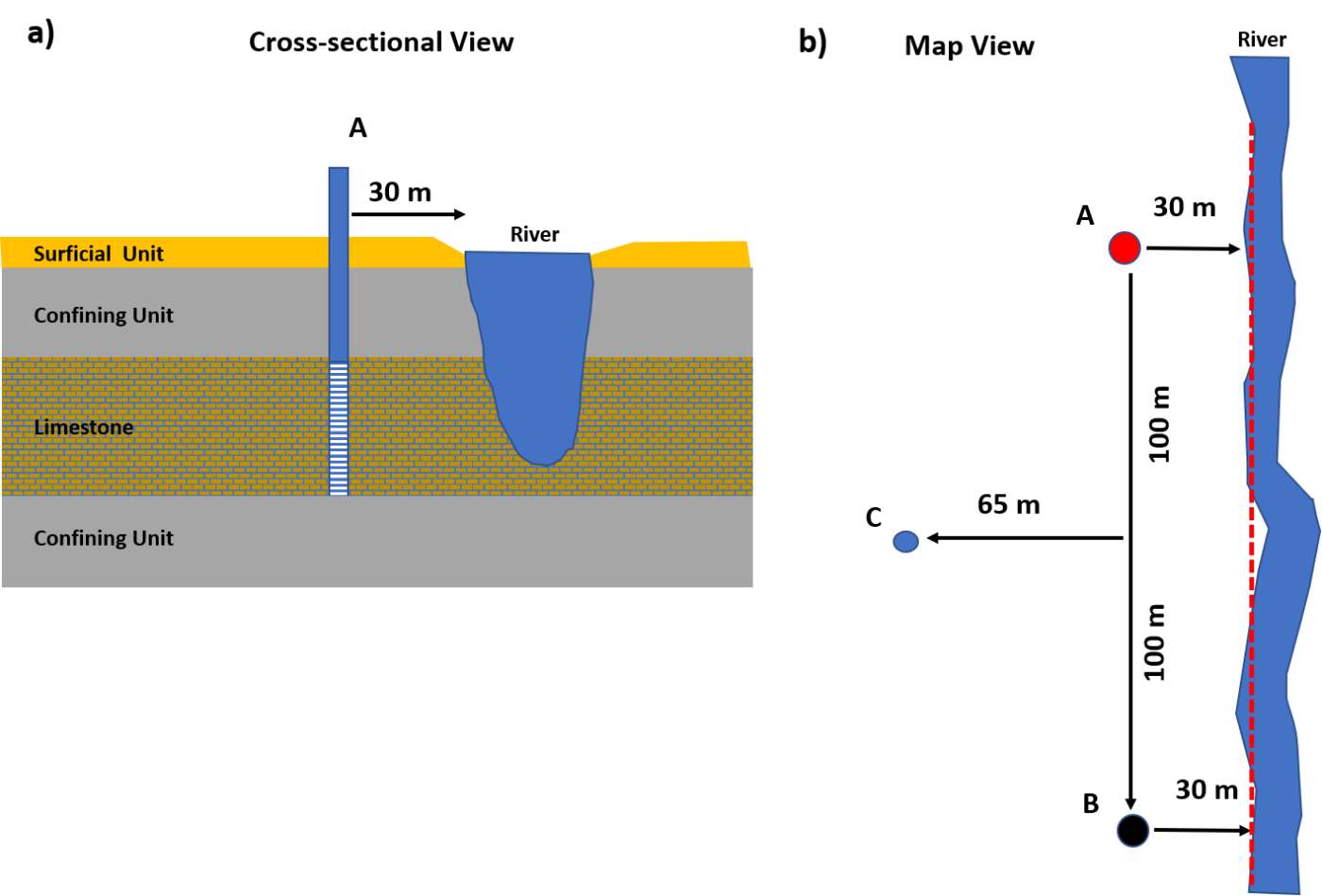
Production wells located near a fully penetrating river. On average, the distance to the river in the confined aquifer is 30 m from the pumping well as shown by the red dashed line. a) Cross section showing production well A and the lithology. b) Map view of the well locations relative to the river.
- Compute the well interference (drawdown) that would occur at B when well A is pumped at 900 m3/d for 50 days.
This problem deals with a linear recharge boundary where the river penetrates the confined aquifer. Using image well theory (Section 11), the river acts as an infinite source of water to the aquifer. To compute the drawdown at well location B the effect of the boundary must be represented by an image well (IA) located 30 m across the boundary from well A. As the image well represents the effects of a recharge boundary it becomes an injection well to mathematically create no drawdown at the boundary (i.e., an injection well has drawup, or negative drawdown) with an inflow of 900 m3/d. The total drawdown at B from pumping A and the effects of the recharge boundary must be considered as shown in the image below.
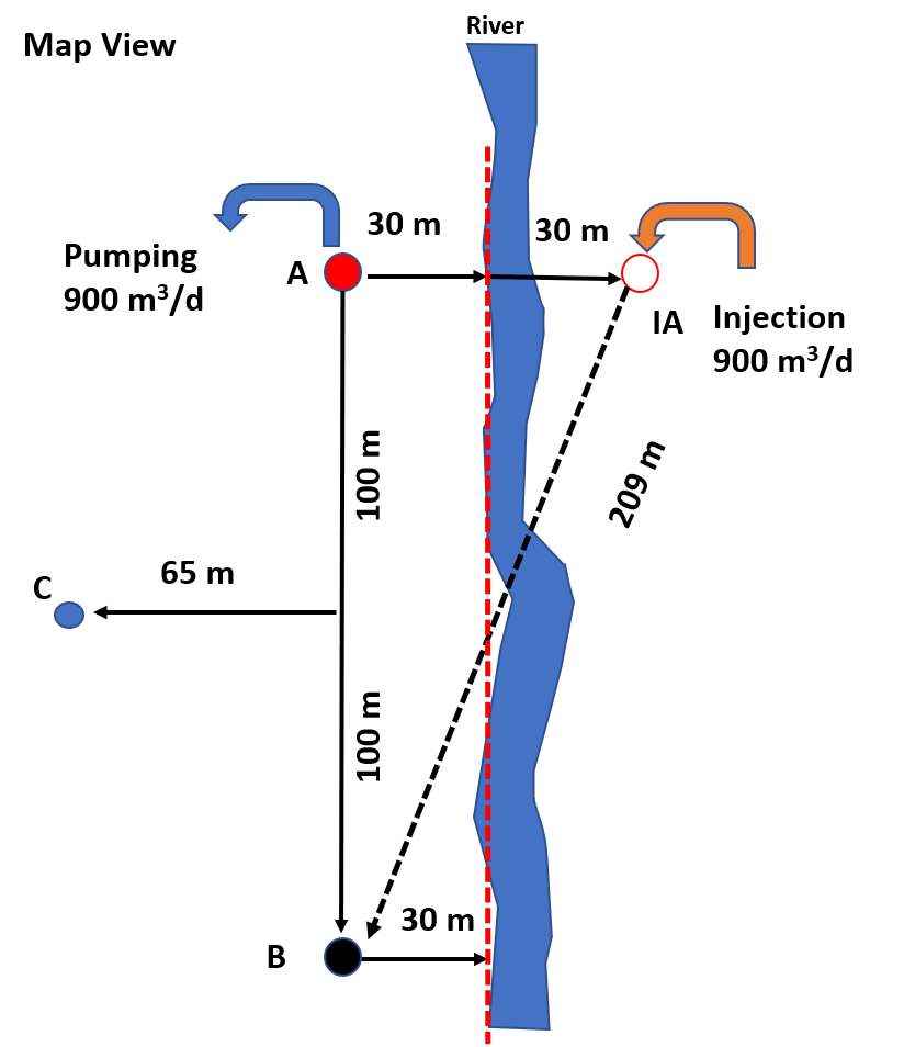
Application of image well theory. Well IA is an image well representing the effect of the linear recharge boundary (river) when A is pumped. The image well is represented by an injection well (‑900 m3/d). The figure also shows the radial distance from image well IA to location B.
[latex]s_{T}\ at\ B = s_{A} + s_{IA}[/latex]
Using the Theis Equation (26), the total drawdown at B can be computed. First, u is calculated, then W(u) is read from Figure 26 and drawdown is calculated using Equation (26).
First, compute u for well A.
[latex]u_{A} = \frac{r^{2}S}{4Tt} = \frac{{(200\ m)}^{2}\ \ 0.00003}{4\left( 75\frac{m^{2}}{d} \right)50\ d} = 0.00008 \cong 8x10^{- 5}[/latex]
Then using Figure 26 to look up, or WolframAlpha to solve W(u)=‑Ei(‑u), W(uA) is ≅ 8.8563.
[latex]s_{A} = \frac{Q}{4\pi T}\ W(u) = \frac{900\ \frac{m^{3}}{d}}{4\ (3.14)\ 75\frac{m^{2}}{d}}\ 8.8563 = 8.46\ m[/latex]
Next, compute u for well IA.
[latex]u_{IA} = \frac{r^{2}S}{4Tt} = \frac{{(209\ m)}^{2}\ \ 0.00003}{4\left( 75\frac{m^{2}}{d} \right)50\ d} = 0.000087 \cong 8.7x10^{- 5}[/latex]
Then using Figure 26, W(uIA) is ≅ 8.7725. As the image well represents a recharge boundary effect the pumping rate is input as –900 m3/d.
[latex]s_{IA} = \frac{Q}{4\pi T}\ W(u) = \frac{- 900\ \frac{m^{3}}{d}}{4\ (3.14)\ 75\frac{m^{2}}{d}}\ 8.7725 = - 8.38\ m[/latex]
The “drawdown” computed is negative because it is draw‑up or a rise in water level in response to injection of water.
[latex]s_{T}\ at\ B = 8.46\ m + ( - 8.38\ m) = 0.08\ m[/latex]
- If during the same 50 days of pumping well A, the well at location B is pumped at 450 m3/d, what would be the drawdown at unpumped observation well C at the end of the 50 days of pumping?
The total drawdown at C would be computed shown here.
[latex]s_{T}\ at\ C = s_{A} + s_{IA} + s_{\mathbf{B}} + s_{IB}[/latex]
Drawdown at C is influenced by the two pumping wells and the two image wells that represent the recharge boundary. The image well locations and corresponding radial distances are shown in the following image.
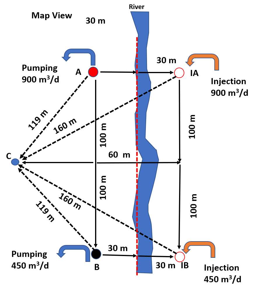
Application of image well theory. Well IA is an image well representing the effect of the linear recharge boundary (river) on the drawdown at A and IB is the image well representing the effect of the boundary on the drawdown at B. To calculate the drawdown at the unpumped well located at C, the effect of all four wells must be considered. The calculated radial distances from pumping and image wells to well C are shown on the figure.
The first step is to compute the radial distances from the pumping and image wells to observation well C. Then values of u are computed for each of the 4 wells and corresponding values of W(u) determined from the table shown in Figure 26 of Section 8. Q for the recharge boundary injection wells is input as a negative rate.
[latex]u_{A} = \frac{r^{2}S}{4Tt} = \frac{{(119\ m)}^{2}\ \ 0.00003}{4\left( 75\frac{m^{2}}{d} \right)50\ d} = 0.000028 \cong 2.8x10^{- 5}[/latex]
Then using Figure 26 to look up, or WolframAlpha to solve W(u)=‑Ei(‑u), W(uA) is ≅ 9.9061.
[latex]\mathbf{s}_{\mathbf{A}} = \frac{Q}{4\pi T}\ W(u) = \frac{900\ \frac{m^{3}}{d}}{4\ (3.14)\ 75\frac{m^{2}}{d}}\ 9.9061 = \mathbf{9.46\ m}[/latex]
[latex]u_{IA} = \frac{r^{2}S}{4Tt} = \frac{{(160\ m)}^{2}\ \ 0.00003}{4\left( 75\frac{m^{2}}{d} \right)50\ d} = 0.000051 \cong 5.1x10^{- 5}[/latex]
Then using Figure 26, W(uIA) is ≅ 9.3065.
[latex]\mathbf{s}_{\mathbf{IA}} = \frac{Q}{4\pi T}\ W(u) = \frac{- 900\ \frac{m^{3}}{d}}{4\ (3.14)\ 75\frac{m^{2}}{d}}\ 9.3065 = \mathbf{- 8.89\ m}[/latex]
[latex]u_{B} = \frac{r^{2}S}{4Tt} = \frac{{(119\ m)}^{2}\ \ 0.00003}{4\left( 75\frac{m^{2}}{d} \right)50\ d} = 0.000028 \cong 2.8x10^{- 5}[/latex]
Then using Figure 26, W(uA) is ≅ 9.9061.
[latex]\mathbf{s}_{\mathbf{B}} = \frac{Q}{4\pi T}\ W(u) = \frac{450\ \frac{m^{3}}{d}}{4\ (3.14)\ 75\frac{m^{2}}{d}}\ 9.9061 = \mathbf{4.73\ m}[/latex]
[latex]u_{IB} = \frac{r^{2}S}{4Tt} = \frac{{(160\ m)}^{2}\ \ 0.00003}{4\left( 75\frac{m^{2}}{d} \right)50\ d} = 0.000051 \cong 5.1x10^{- 5}[/latex]
Then using Figure 26, W(uIB) is ≅ 9.3065.
[latex]\mathbf{s}_{\mathbf{IB}} = \frac{Q}{4\pi T}\ W(u) = \frac{- 450\ \frac{m^{3}}{d}}{4\ (3.14)\ 75\frac{m^{2}}{d}}\ 9.3065 = \mathbf{- 4.45\ m}[/latex]
[latex]\mathbf{s}_{\mathbf{T}}\mathbf{\ at\ C} = s_{A} + s_{IA} + s_{\mathbf{B}} + s_{IB} = 9.46\ m + ( - 8.89\ m) + 4.73\ m + ( - 4.45\ m) = \mathbf{0.85\ m}[/latex]