
8.1 Formulation of the Theis Equation
Development of the Theis analytical solution incorporates the general assumptions described in Section 6.3 along with the following additional assumptions:
- The confined unit is covered by overlying and underlying confining beds that are aquifuges (non‑porous and impermeable, i.e., not permitting any water to leak into the aquifer).
- The source of all water pumped from a well is derived from the instantaneous release of water from elastic storage of the unit (there is no recharge or flow of water into the cone of depression from other sources).
- The pumping well has an infinitesimal diameter.
Figure 24 illustrates the Theis conceptual model.
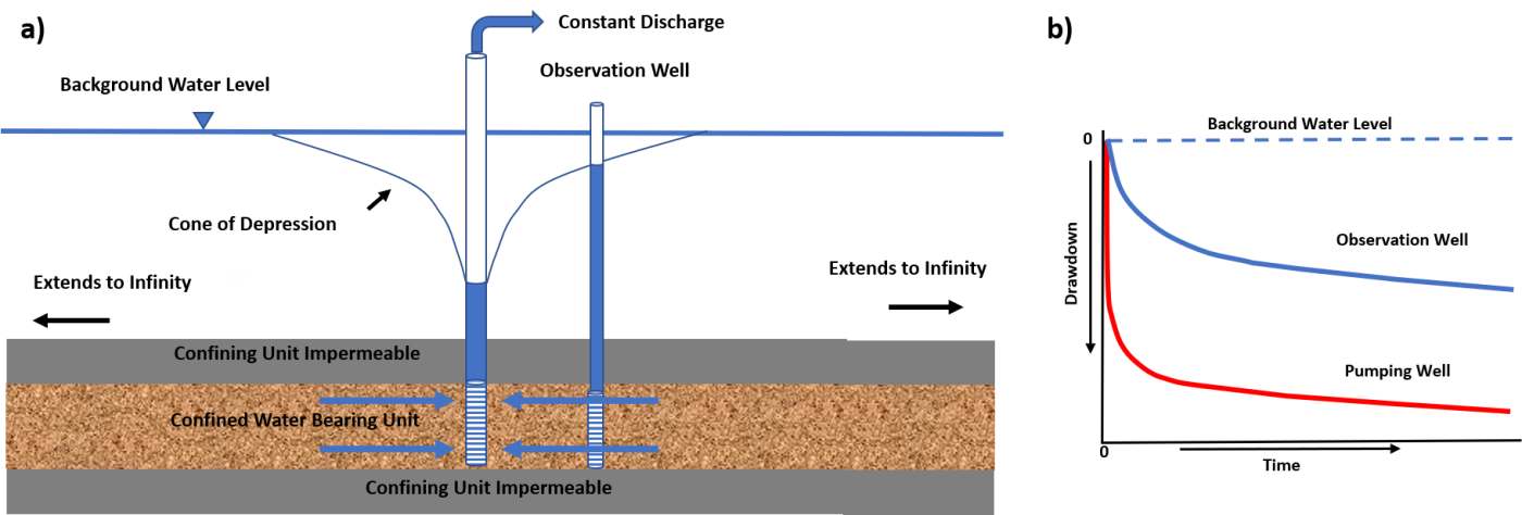
Figure 24 – Conceptual model of the Theis equation conditions describing the head response to pumping in a totally confined isotropic and homogeneous aquifer. a) Cross sectional view of a confined water bearing unit that is infinite in lateral extent as well as overlain and underlain by confining units that are impermeable. b) Schematic of the response of water level changes (drawdown from the corrected‑static water level) in the pumping well and an observation well when the pumping rate is constant.
The basic differential equation, Equation (6), governing radial flow to a well in a confined systems expressed in terms of drawdown is repeated here for the reader’s convenience (Loaiciga, 2009).
| [latex]\frac{S}{T}\frac{\partial s}{\partial t} = \frac{1}{r}\frac{\partial s}{\partial r} + \left( \frac{\partial^{2}s}{\partial r^{2}} \right)[/latex] | (24) |
|---|
where:
| s | = | drawdown, corrected pre‑pumping static head minus head at time t (L) |
|---|---|---|
| r | = | radial distance from the center of the pumped well to the observation well (L) |
| t | = | elapsed time since the start of pumping (T) |
| T | = | transmissivity (L2T‑1) |
| S | = | storativity (dimensionless) |
Equation (24) can be visualized by describing the transient radial flow in any cylindrical section within the cone of depression of a confined system (Figure 25).
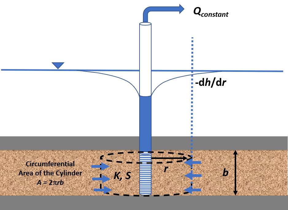
Figure 25 – Conceptualization of confined radial flow in the cone of depression during pumping at a constant rate, Q. The water bearing unit is shown in tan and the impermeable confining beds in gray. The tan patterned saturated material of thickness b is totally confined (gray confining beds). The radial discharge of groundwater, Q, through a cylinder of aquifer is shown by the blue arrows, r is the radius of the cylinder, b is the aquifer thickness, K is the hydraulic conductivity, S is the storativity, and ‑dh/dr is the hydraulic gradient at the outer edge of the cylinder (blue dashed line). Q is equal to the product of the flow velocity at distance r from the well and the circumferential cross‑sectional area (2πrb) so Q = ‑2πrbK (dh/dr). As pumping progresses ‑dh/dr varies with time and water is released from storage, S (‑dh/dt).
Using the basic confined radial‑flow differential equation, general mathematical assumptions presented in Section 6.3, and the additional assumptions that support the Theis equation, along with specified initial and boundary conditions, an analytical solution describing the expected drawdown, s, within the cone of depression at any time after constant pumping begins was derived. Conditions include that drawdown is zero at the start of the pumping. Given that h(r,t) is the head at a radial distance and time, then h(r,0) = h0 = 0 for all r, where h0 is the corrected‑static head. The condition that the confined formation has infinite lateral extent is given by h([latex]\infty[/latex],t) = h0 for all t. The constant pumping rate is represented as a point sink at r = 0. It represents the well, which is a vertical line through the aquifer, but the two‑dimensional aquifer can be represented by a one‑dimensional equation given that the well fully penetrates a homogeneous horizontal layer such that at any radius (r) the drawdown is the same at all vertical positions in the aquifer. All in all, the differential equation accounting for flow and the release of water from storage as the heads change is generated using calculus techniques that are quite involved and are not described here but can be found in Loaiciga (2009).
The Theis solution formulated in terms of drawdown, s, is presented in Equation (25). The integral in Equation (25) is known as the exponential integral. Methods to approximate this integral are known and have been compiled in tables for corresponding values of the argument, u = r2S/(4Tt). When computing u, units should result in a value of u that is dimensionless. Equation (25) is commonly written as Equation (26) with W(u) inserted to represent the Theis well function (i.e., the exponential integral).
| [latex]s(r,t) = \frac{Q}{4\pi T}\ \int_{\frac{r^{2}S}{4Tt}}^{\infty}{\ \frac{1}{y}\ \exp( - y)}\ dy[/latex] | (25) | |
|---|---|---|
| [latex]s(r,t) = \frac{Q}{4\pi T}\ W(u)[/latex] | (26) |
where:
| s(r,t) | = | drawdown at a radial distance r and time t (L) |
|---|---|---|
| Q | = | constant well discharge rate (L3T‑1) |
| T | = | transmissivity (L2T‑1) |
| S | = | storativity (dimensionless) |
| t | = | time (T) |
| r | = | radial distance (L) |
| W(u) | = | Theis well function (dimensionless) |
| u | = | r2S/(4Tt) (dimensionless) |
A solution for the well function, W(u) = [latex]\left\lbrack \ - 0.5772 - \ln u + u - \frac{u^{2}}{2 \bullet 2!} + \frac{u^{3}}{3 \bullet 3!} - \frac{u^{4}}{4 \bullet 4!} + \ldots \right\rbrack[/latex] is an infinite series in which values in the sequence become smaller and smaller as the components are computed. Equation (27) shows the substitution for W(u). Most often values of W(u) are rounded to a few decimal places and only the first three or four terms of the well function equation are required to determine W(u). Tables of the well function computed for values of u are readily available in the literature and can be obtained on the internet (e.g., Figure 26).
| [latex]s = \ \frac{Q}{4\pi T\ }\ \left\lbrack \ - 0.5772 - \ln u + u - \frac{u^{2}}{2 \bullet 2!} + \frac{u^{3}}{3 \bullet 3!} - \frac{u^{4}}{4 \bullet 4!} + \ldots \right\rbrack[/latex] | (27) |
|---|
where:
| s | = | drawdown (L) |
|---|---|---|
| Q | = | constant well discharge rate (L3T‑1) |
| T | = | transmissivity (L2T‑1) |
| u | = | r2S/(4Tt) (dimensionless) |
| t | = | time (T) |
| r | = | radial distance (L) |
| S | = | storativity (dimensionless) |
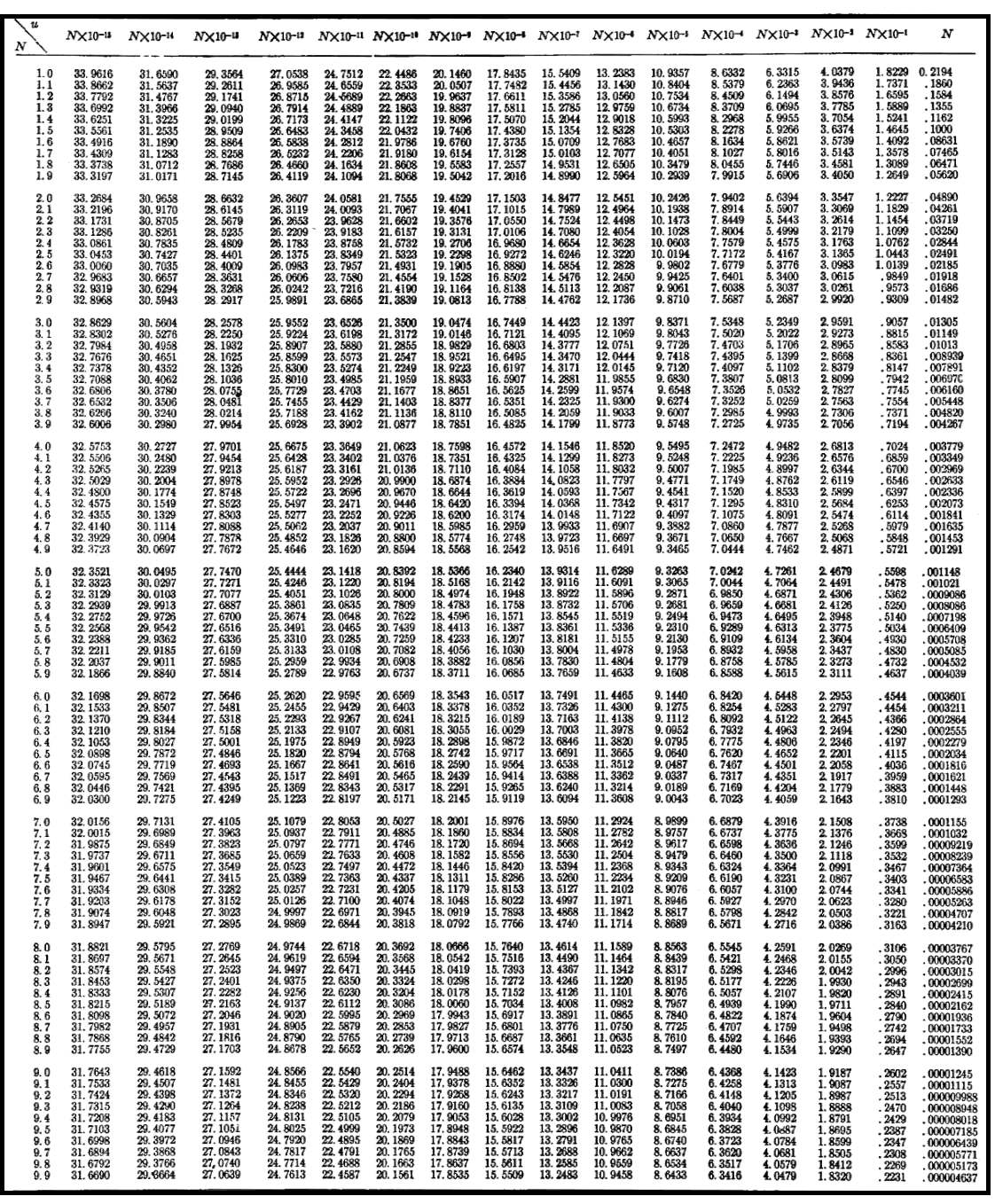
Figure 26 – Table of u(N) and corresponding W(u) values. Values of u are found on the left‑hand vertical column (1.0‑9.9). The top of the table represents u multiplied by values of 10‑15 to 100 with the right‑hand column being values of W(u) for u multiplied by 1. For example, if u = 4.6 x 10‑9 one would find the value of 4.6 in the left column and then scan right to find the value under the column labeled Nx10‑9, where W(u) equals 18.62. Tables like this one are found in many introductory hydrogeology textbooks. This table comes from Lohman (1972).
The table (Figure 26) provides one way to obtain the Theis well function for a computed value of u. When u values do not match table u values, they are often estimated using linear interpolation between corresponding table values. As the relationship between u and W(u) is non‑linear a more precise method is to compute W(u) using the representation shown in Equation (27). Use of the table shown in (Figure 26) can be avoided and easily replaced by directly computing a value of W(u) from values of u. For example, the well function can be written as or W(u) = ‑Ei(‑u) and a number of mathematics software programs can be used to obtain the value. A free option is to use the WolframAlpha.com equation solver↗ on the Internet as shown in Figure 27.
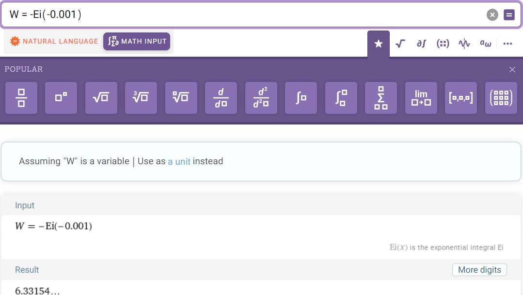
Figure 27 ‑ Use of the WolframAlpha.com equation solver↗ on the Internet to determine the value of W(u). The result for u= 0.001 is 6.3315 which is the same value shown in the table of Figure 26.
The relationship between W(u) and u is such that as u becomes smaller as W(u) becomes larger. A log‑log plot of what is referred to as the Theis type curve is created by plotting values W(u) on a vertical log axis and values of 1/u on the horizontal log axis. Figure 28 shows the inverse relationship of u and W(u) because W(u) increases with an increase in 1/u (Figure 28). A log‑log plot of drawdown data versus time from a field test has the same form.
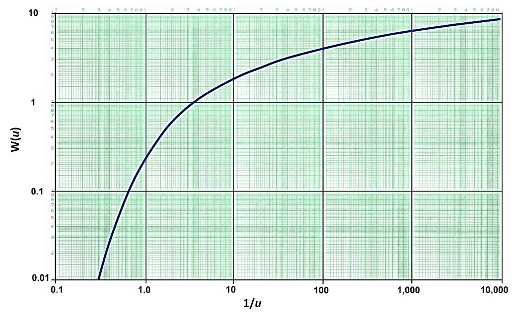
Figure 28 ‑ The Theis type curve is a log‑log plot of the Theis well function W(u) for corresponding values of 1/u.
The type curve can also be plotted as a log‑log plot as W(u) versus u. In that case, field data are plotted as s versus r2/t. This representation is used by some hydrogeologists when interpreting pumping test data (e.g., Lohman, 1972). Type curves in this book are plotted as W(u) versus 1/u which takes the same form as a plot of drawdown versus time, s versus t.
When a pumping test is conducted in a confined aquifer, the time‑drawdown response is dependent on the relative values of T and S. The drawdown at a radial distance from the pumping well is inversely proportional to T and directly proportional to the pumping rate as shown in Equation (27). The relationship to S is more difficult to discern because it is inside the expression for u, but drawdown at a radial distance from the pumping well is also inversely proportional to S. For similar magnitudes of change, transmissivity has a greater influence on the total drawdown than the storativity. Figure 29 illustrates how the cone of depression profile varies under selected combinations of T and S. For a given value of S, when T increases the drawdown cone becomes broader and shallower. For a given value of T, when S increases the drawdown cone becomes narrower and deeper. Generally, as T and S increase, the cone of depression becomes shallower, whereas when T and S values decrease, the cone of depression expands and becomes deeper. These observations are useful when developing conceptual models of the likely behavior of a confined groundwater system to pumping.
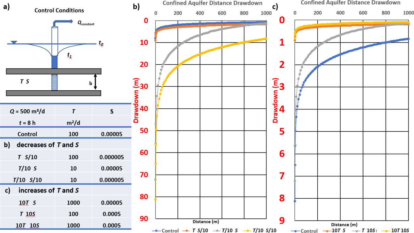
Figure 29 – Illustration of the influence of T and S on the shape and extent of drawdown when pumping an isotropic and homogeneous confined aquifer at a constant rate of 500 m3/d and observing drawdown versus distance from 0 to 1,000 m after 8 hours of pumping. Drawdown extends beyond 1,000 m after 8 hours of pumping, but the graph was truncated at 1000 m for this illustration. The pumping well is located at r = 0.
a) Schematic of the control conditions and a table of the assigned variations of the control settings. A designation such as T,S/10 corresponds to the control value of T and the reduction of S by an order of magnitude, S/10.
b) Comparison of the effect of reducing T and S by an order of magnitude plotted along with the control conditions (blue line). The vertical scale is from 0 to 90 m, and in red to help the reader notice the scale change between (b) and (c). When T and S are smaller than the control values the drawdown versus distance profile is deeper and extends further beyond the 1,000 m which is the maximum value of r that is plotted here (so there is more drawdown at r = 1,000 m than for the control drawdown).
c) Comparison of the effect of increasing T and S by an order of magnitude plotted along with the control conditions (blued line). The vertical scale is from 0 to 9 m, much smaller than that of (b), and in red to help the reader notice the scale change between (b) and (c). As T and S values increase relative to the control values, the drawdown distance profile is shallower with less drawdown at the 1,000 m x‑axis terminus. Drawdown versus time values were simulated using AQTESOLV V5, www.aqtesolv.com↗.
Section 8.2 addresses the use of the Theis analytical solution and aquifer parameters to predict drawdown.