
10.4 Computing T and S from Aquifer Test Data
Curve matching and numerical methods are used to match field time‑drawdown data with analytical solutions that use ua, uy, η and W(ua,uy,η). Curve matching techniques described in Section 8.3.1 are applicable here. Neuman’s representation of the instantaneous release of water from storage assumptions result in poor values of S that are usually higher than the field value of the early‑time confined storage, and lower than the field value for the late‑time specific yield. The transmissivity values obtained using Neuman’s techniques are considered representative of field properties. Nwankwor and others (1992) recommend Sy should only be computed from late time test data citing the need for at least a three‑day pumping test.
Again, to build a basic understanding of the methods used to analyze field data, a description of the manual approach is presented in this section. When the values in Figure 60 and Figure 61 are plotted on log‑log scales a family of curves is created. These type curves are a bit complicated, as values of W(ua,uy,η) are plotted on the vertical axis, values of 1/ua are plotted on the top x axis, values of 1/uy are plotted on the lower x axis, and a family of curves are derived for values of η. In addition, the Theis curves for confined conditions (S) and unconfined conditions (Sy) are also plotted (Figure 62).
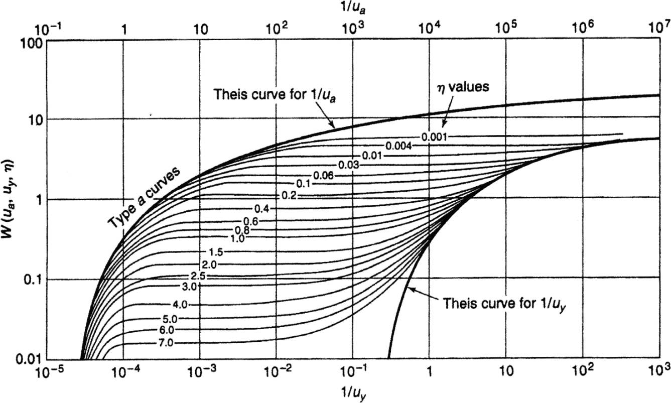
Figure 62 ‑ Neuman type curves for unconfined systems with delayed yield (Todd and Mays, 2005).
When a delayed yield is observed in drawdown data from an unconfined pumping test (Figure 63), curve matching is a two‑step process (Figure 64 and Figure 65).
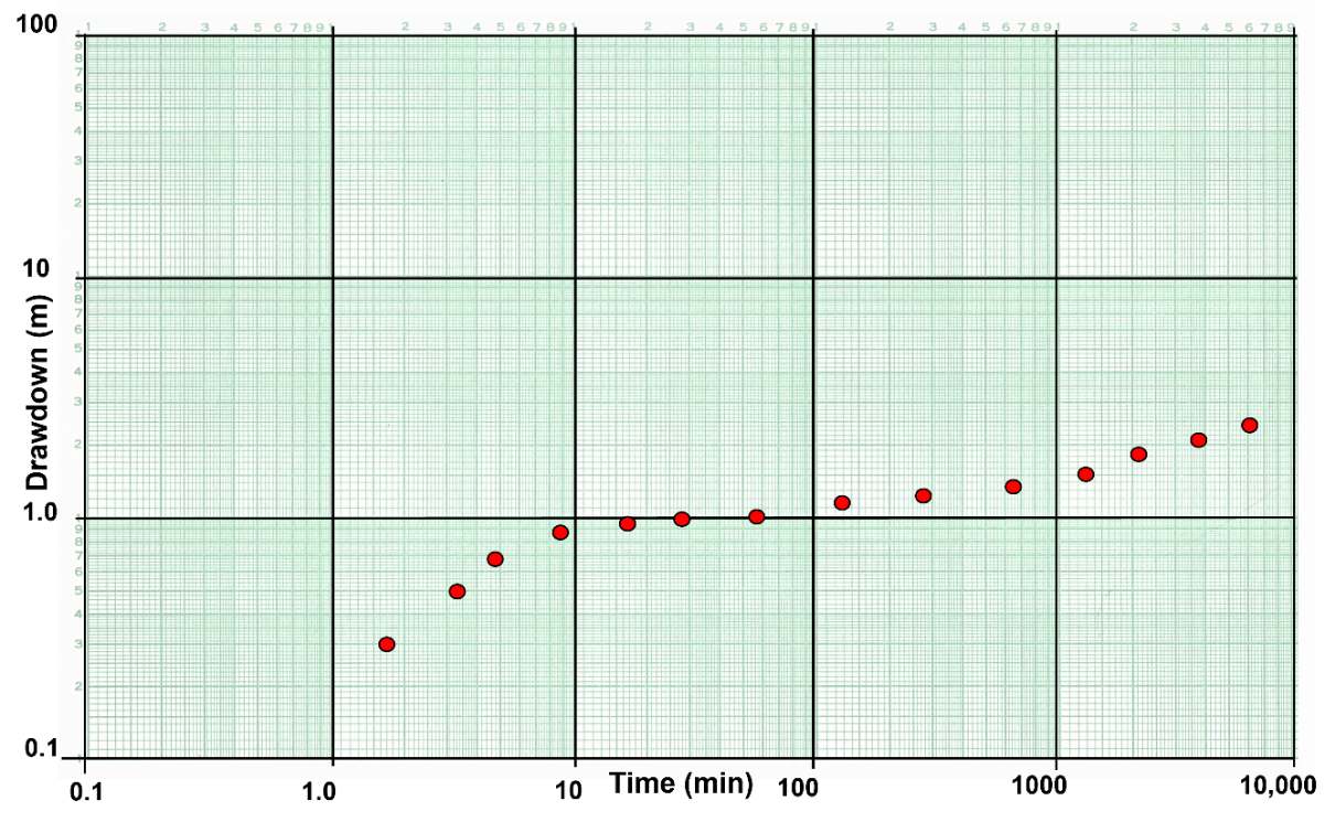
Figure 63 ‑ An example of a log‑log time‑drawdown plot of field data (solid red dots) collected at an observation well in an unconfined aquifer being pumped at a constant rate.
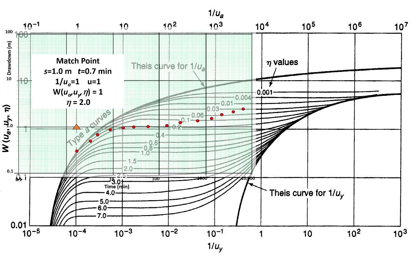
Figure 64 ‑ Matching early time‑drawdown data with Neuman’s (1975) unconfined delayed yield type curves.
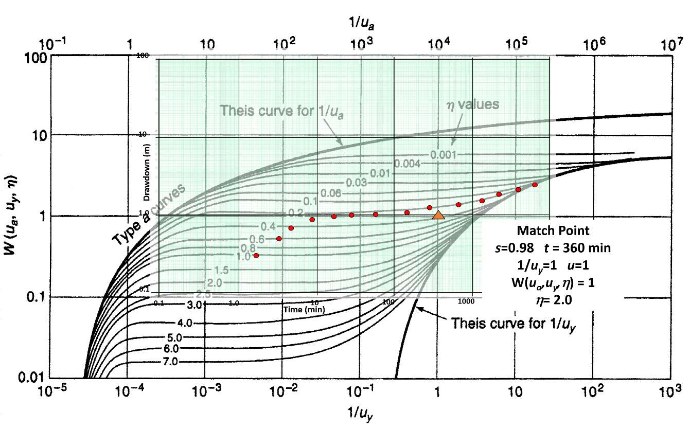
Figure 65 ‑ Matching late time‑drawdown data with Neuman’s (1975) unconfined delayed yield type curves.
Standard curve matching procedures are applied. Plots are prepared using identical log‑log scales and axes are kept parallel. The first step is to match the early‑time data with the left‑hand portion of Figure 62. A match point is selected using the top x‑axis (1/ua) and the left vertical scale (W(ua,uy,η). Then s and t values are obtained from the drawdown plot, and the η curve value is noted (Figure 64). When delayed yield is affecting the drawdown data, the complete type curve plot (Figure 64) is not treated as continuous because the periods of delayed yield are variable and aquifer specific. The second step is to slide the data plot to the right along the η curve used to match the early data and determine the best match to the late time data (Figure 65). The data matches should be on the same η curve. The late‑time data are matched, and a second match point is selected. The late‑time match point includes 1/uy taken from the lower x‑axis, W(ua,uy,η) from the vertical axis, s and t from the time‑drawdown curve, and the value of the η curve.
When T is calculated for both the early‑ and late‑time data, values are usually very similar. Values are averaged to determine a representative value. As stated earlier, S values are often poorly represented (as shown in the example below). Thus, storage values obtained by curve matching are often replaced with lab or literature‑derived values are used to represent the unconfined aquifer instead of computed values (e.g., Box 2 of this book, as well as Woessner & Poeter, 2020). Analyzing time drawdown data for an extended period after the delayed‑yield portion of the response dissipates is recommended to generate more representative specific yield values form late‑time data.
Transmissivity is computed by rearranging Equation (70) to Equation (74). Storativity values are calculated by solving for S and Sy in Equations (71) and (72). The horizontal hydraulic conductivity can be estimated as T/b and the vertical hydraulic conductivity can be obtained by rearranging Equation (73) to Equation (78).
| [latex]T = \frac{Q}{4\pi s}\ W\left( u_{a},u_{y,}\eta \right)[/latex] | (74) | |
|---|---|---|
| [latex]\frac{u_{a}4Tt}{r^{2}} = S[/latex] | (75) | |
| [latex]\frac{u_{y}4Tt}{r^{2}} = S_{y}[/latex] | (76) | |
| [latex]\frac{T}{b} = K[/latex] | (77) | |
| [latex]\frac{\eta b^{2}K_{h}}{r^{2}} = K_{z}[/latex] | (78) |
where:
| s(r,t) | = | drawdown at a radial distance r and time t (L) |
|---|---|---|
| Q | = | constant well discharge rate (L3T‑1) |
| T | = | transmissivity (L2T‑1) |
| S | = | storativity under early time confined conditions (dimensionless) |
| Sy | = | storativity at late times, specific yield (dimensionless) |
| t | = | time (T) |
| r | = | radial distance to the observation well (L) |
| ua | = | early time values of u (dimensionless) |
| uy | = | late time values of u (dimensionless) |
| W(ua,uy,η) | = | unconfined well function (dimensionless) |
| Kz | = | unconfined vertical hydraulic conductivity (LT‑1) |
| Kh | = | unconfined horizontal hydraulic conductivity (LT‑1) |
| b | = | pre‑pumping saturated thickness (L) |
| η | = | variable defined by Equation (73) (dimensionless) |
Example
T, S, and Sy can be estimated using the match points (Figure 64 and Figure 65) if it is assumed that the data represented in Figure 63 were collected at an observation well located 120 m from the pumping well during a 4‑day hydraulic test with a well pumping at 4,000 m3/d. The aquifer has a pre‑pumping saturated thickness of 28 m and is sand and gravel. Match point data in Figure 64 are used to compute the transmissivity from early‑time data using Equation (74) and storativity using Equation (75).
[latex]T = \frac{4000\frac{m^{3}}{d}}{4\ (3.14)\ 1\ m}\ (1) = 318\frac{m^{2}}{d}[/latex]
[latex]S = \frac{(1)\ 4\ \left( 318\frac{\ m^{2}}{d} \right)0.0005\ d}{{(120\ m)}^{2}} = 0.000044\ \ or\ \ 4.4{x10}^{- 5}[/latex]
Using the late time match point of Figure 65 and Equations (74) and (76), transmissivity and specific yield are calculated.
[latex]T = \frac{4000\frac{m^{3}}{d}}{4\ (3.14)\ 0.98\ m}\ (1) = 325\frac{m^{2}}{d}[/latex]
[latex]S_{y} = \frac{(1)\ 4\ \left( 325\frac{\ m^{2}}{d} \right)\ 0.25\ d}{{(120\ m)}^{2}} = 0.02[/latex]
Averaging the T values yields a value of 322 m2/d. In this example the confined storage coefficient seems reasonable, but the specific yield is quite small and most likely not representative of field conditions. This suggests that analytical formulations may not fully capture the release of water as the aquifer dewaters.
The horizontal hydraulic conductivity is computed using Equation (77)
[latex]\frac{322\frac{\ m^{2}}{d}}{28\ m} = 11.5\ \frac{m}{d}[/latex]
Next using Equation (78) and match point value of η =2.0, vertical hydraulic conductivity is calculated.
[latex]K_{z} = \frac{(1)\ 2.0\ {(28\ m)}^{2}\ \ 11.5\ \frac{m}{d}}{{(120\ m)}^{2}} = 1.3\frac{m}{d}[/latex]
Analytical approaches to describing the response of wells when pumping an unconfined system were outlined in this section. Numerical methods can also be used to approximate the response of unconfined aquifers to pumping. However, representation of delayed yield processes requires additional model complexity (e.g., Anderson et al., 2015; Diersch, 2014).
Section 11 presents methods to assess how boundaries, well interference, and anisotropy affect efforts to forecast drawdowns and estimate hydrogeologic properties.