
7.1 Steady‑State Conditions in a Confined Groundwater System
The general assumptions listed under the discussion of the development of analytical solutions in Section 6 are applied when developing equations to represent steady‑state pumping conditions. An additional condition is applied stating that drawdown has reached equilibrium as the cone of depression ceases to expand as pumping continues.
The steady‑state mathematics are based on Darcy’s Law and the conservation of mass. Under steady‑state conditions the gradients within the cone of depression do not change over time. With radial flow, the discharge at any given radial distance from the pumping well is equal to the hydraulic conductivity (K) times the cross‑sectional area (2πrb), times the gradient (‑dh/dr) at that radial distance from the pumping well (Figure 18).
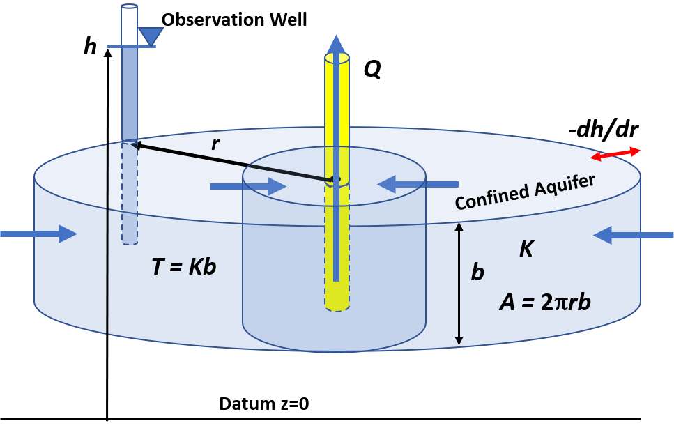
Figure 18 – The radial flow of water through a cylindrical area within the steady‑state cone of depression in an isotropic and homogeneous system. The well discharge, Q, is constant as it passes through each circumferential cross‑sectional area, A, defined as 2πrb. The hydraulic conductivity is represented by K. The steady‑state gradient (‑dh/dr) is constant at each r.
Darcy’s Law is the equation describing steady‑state flow in an isotropic and homogeneous confined aquifer as shown in Equation (16).
| [latex]\frac{dh}{dr} = \frac{Q}{2\pi Tr}[/latex] | (16) |
|---|
where:
| h | = | total head measured from a datum (L) |
|---|---|---|
| r | = | radial distance to an observation well (L) |
| Q | = | constant pumping rate, negative for withdrawal (L3T‑1) |
| T | = | confined aquifer transmissivity (Kb) (L2T‑1) |
| K | = | hydraulic conductivity (LT‑1) |
| b | = | thickness of the confined aquifer (L) |
Equation (16) is used to generate an analytical solution when it is constrained by conditions where the heads at two observation wells, each located at a different radial distance from the pumping well, are known as shown in Figure 19. Standard integration techniques are used to derive what is referred to the Thiem steady‑state equation for pumping a confined unit.
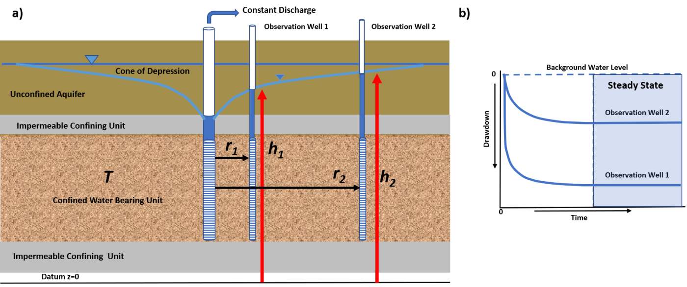
Figure 19 – Cross section of a confined aquifer and the parameters used to define steady‑state conditions. a) The heads at the observation wells (red arrows) are measured from a datum. The radial distances are measured from the pumping well. b) An arithmetic plot of drawdown and time showing the drawdown reaching steady‑state conditions (dashed vertical black line and blue shaded area).
The Thiem analytical solution (Thiem, 1906) for a confined aquifer is written in terms of transmissivity as shown in Equation (17).
| [latex]T = \frac{Q}{2\pi\left( h_{2} - h_{1} \right)}\ln\left( \frac{r_{2}}{r_{1}} \right)[/latex] | (17) |
|---|
where:
| T | = | confined aquifer transmissivity (Kb) (L2T‑1) |
|---|---|---|
| Q | = | constant pumping rate (L3T‑1) |
| h2 | = | head at observation well 2 located further from the pumping well (L) |
| h1 | = | head at observation well 1 located closer to the pumping well (L) |
| r2 | = | radial distance to observation well 2 (L) |
| r1 | = | radial distance to observation well 1 (L) |
Equation (17) does not include storativity of the aquifer because storage is irrelevant in a steady‑state system as indicated by the steady‑state groundwater flow equations. In a steady‑state system, the heads are constant and no water is released from storage during pumping. The equation can be used to solve for T when a constant‑discharge test includes drawdown data from two observation wells.
Example
Let us assume there is a well in a confined groundwater system pumping at 1,500 m3/d and the heads have stopped declining after some time signaling steady‑state conditions are occurring. If the head in observation well 1 at a radial distance of 55 m is 1,033 m and the head at observation well 2 at a radial distance of 150 m is 1,040 m, compute T.
[latex]T = \frac{1,500\ \frac{m^{3}}{d}}{2\ (3.14)\ (1040m - 1033m)}\ ln\frac{150\ m}{50\ m}\ = \ 37.5\frac{m^{2}}{d}[/latex]
The Thiem equation can also be used to predict the steady‑state head at an observation well located at any radial distance from the pumping well if the aquifer transmissivity, pumping rate, head, and the radial distance to one observation well are known.