
10.1 Approximating the Response of Pumping Unconfined Aquifers Using Theis Approach
As illustrated in Figure 56, time‑drawdown data in unconfined units will sometimes mirror the Theis type curve response. For example, in an isotropic and homogeneous high hydraulic conductivity system with large pore spaces being pumped at a rate that results in a small reduction in saturated thickness, drawdown is likely to mirror a Theis‑like response.
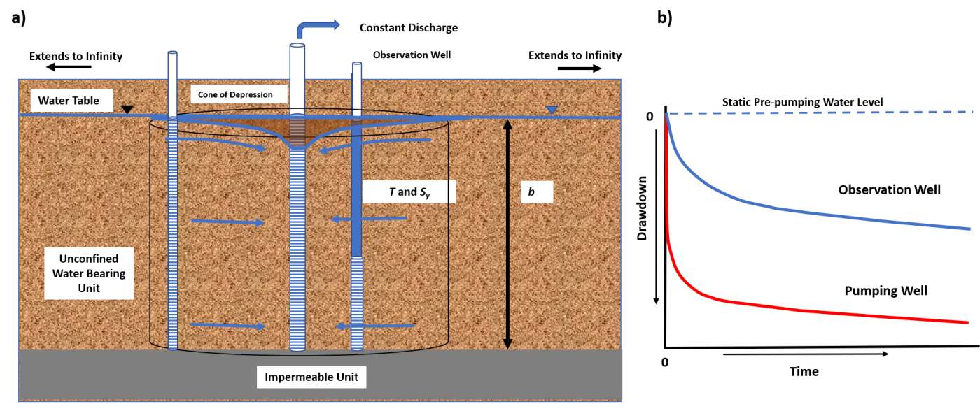
Figure 56 ‑ Conceptual model of the response of an isotropic and homogeneous coarse‑grained unconfined water‑bearing unit to constant pumping. The volume of the cone of depression affected at a specific time is represented by the cylinder. The initial saturated thickness is b. The volume dewatered is shown in brown. A) In this setting the coarse nature of the material is such that the capillary fringe is small, and the release of gravity‑drained water added to the declining water table is instantaneous. B) The arithmetic drawdown response mirrors the Theis logarithmic decline.
The analytical equation describing the resulting drawdown behavior is the Theis equation (Theis, 1935) shown here as (64). If the formational properties (T and Sy) are known, drawdown at any location and time can be computed using Equation (64). To compute u the confined storativity is replaced with the unconfined storativity (Equation (65), Sy (discussed in detail in Box 2).
| [latex]s(r,t) = \frac{Q}{4\pi T}\ W(u)[/latex] | (64) | |
|---|---|---|
| [latex]u = \frac{r^{2}S_{y\ }}{4Tt}[/latex] | (65) |
where:
| s(r,t) | = | drawdown at a radial distance r and time t (L) |
|---|---|---|
| Q | = | constant well discharge rate (L3T‑1) |
| T | = | transmissivity (L2T‑1) |
| t | = | time (T) |
| W(u) | = | Theis well function (dimensionless) |
| Sy | = | unconfined storativity (specific yield) (dimensionless) |
The predicted drawdown is considered representative if the degree of aquifer dewatering at the prescribed radial distance from the pumping well is small, less than 10 percent (Kasenow, 2001; USDI, 1981).
Example
If an unconfined aquifer with T= 300 m2/d and Sy = 0.08 is pumped at 1,000 m3/d for 0.5 days, compute the drawdown at 100 m from the pumping well. The pre‑pumping saturated thickness of the unconfined aquifer is 25 m. Equation (65) is used to compute u and then the Theis well function is determined from the table shown in Figure 26.
[latex]u = \frac{{(100\ m)}^{2}\ 0.08}{4\ \left( 300\frac{\ m^{2}}{d} \right)\ 0.5\ d} = 1.33[/latex]
This value of u falls outside of the range of the table in Figure 26, however the value is readily obtained using the WolframAlpha.com equation solver↗ on the Internet as shown in Figure 27 where W(1.33) is found to be 0.13 and s can be calculated as follows.
[latex]s = \frac{1000\frac{\ m^{3}}{d}}{4\ (3.14)\ 300\frac{\ m^{2}}{d}}\ 0.13 = 0.035\ m[/latex]
Next, we check whether the predicted drawdown values need to be corrected. If they are less than 10 percent of the initial aquifer thickness, then correction is not needed.
[latex]percent\ thickness\ = \ \frac{0.035\ m}{25\ m}\ (100) = \ 0.14\ percent[/latex]
Less than 10 percent of the aquifer is dewatered at this location, so no drawdown correction is needed.
In some cases, drawdown due to pumping in an unconfined unit measurably reduces the saturated thickness, yet no delayed yield is observed. In these settings T varies spatially and temporally due to the substantial differences in thickness, b=h, and T=Kb. Drawdown predicted by the unconfined Theis equation is less (drawdown values are smaller) than what would occur in the field for an unconfined system experiencing significant reduction of saturated thickness. Jacob (1950) suggested that the predicted drawdowns should be corrected to represent the actual drawdown that would occur with significant dewatering. He recommended that a correction was needed if the ratio of drawdown to the initial saturated thickness was greater than 0.02. This value is more conservative than the 10 percent guidance by the UDSI (1981). Schwartz and Zhang (2003) present a method to correct the computed drawdown. The resulting corrected drawdown value will be greater than the Theis equation computed value.
| [latex]s = b - (b^{2} - 2s'b)^{0.5}[/latex] | (66) |
|---|
where:
| s | = | corrected drawdown for the unconfined aquifer (L) |
|---|---|---|
| s’ | = | drawdown computed using the standard Theis method (L) |
| b | = | pre‑pumping saturated thickness of the unconfined aquifer (L) |
Example
The Theis equation is used to estimate the drawdown, 5.6 m, at an observation well located 150 m from a well pumping at 600 m3/d. The pre‑pumping saturated thickness was 30 m. Because some dewatering occurs, 5.6 m/30 m = 0.19, the resulting final water table drawdown would be derived using Equation (66).
s[latex]= 30\ m - ({(30\ m)}^{2} - (2\ (5.6\ m)\ (30\ m))^{0.5} = 6.25\ m[/latex]
Pumping Test Analysis
When a pumping test of this type of unconfined system is conducted, curve matching methods as described in Section 8 are applied. If dewatering is less than 10 percent during a pumping test—or, using Jacob’s (1950) recommendation, is less than s/b =0.02—then standard curve matching methods using the Theis type curve can be performed using Equations (67) and (68).
| [latex]T = \frac{Q}{4\pi s}\ W(u)[/latex] | (67) | |
|---|---|---|
| [latex]S_{y} = \frac{u4Tt}{r^{2}}[/latex] | (68) |
where:
| T | = | transmissivity (L2T‑1) |
|---|---|---|
| Q | = | constant pumping rate (L3T‑1) |
| s | = | drawdown (L) |
| W(u) | = | Theis well function (dimensionless) |
| Sy | = | specific yield unconfined storage coefficient (dimensionless) |
| u | = | integral argument (dimensionless) |
| t | = | time (T) |
| r | = | radial distance to pumping well (L) |
However, if during a pumping test significant dewatering occurs at observation points drawdowns need to be corrected before a Theis curve matching approach is applied. Again, this is because with a reduction in saturated thickness more drawdown occurs than if the aquifer remained fully saturated during the test (constant T) because the reduced thickness reduces T. This correction was described by Jacob (1963) and in Section 7 of this book. It is shown here as Equation (69). The correction is valid for conditions where 10 to 25 percent of saturated thickness dewaters during the test (Kasenow, 2001). Once the data set is corrected it can be used to generate a drawdown time curve, after which a Theis curve matching analysis is performed.
| [latex]s_{c} = s - \frac{s^{2}}{2b}[/latex] | (69) |
|---|
where:
| sc | = | corrected unconfined drawdown (L) |
|---|---|---|
| s | = | measured drawdown during the unconfined pumping tests (L) |
| b | = | initial saturated thickness (L) |
Example
An example of unconfined pumping test results that mirrors the Theis model is shown in Figure 57.
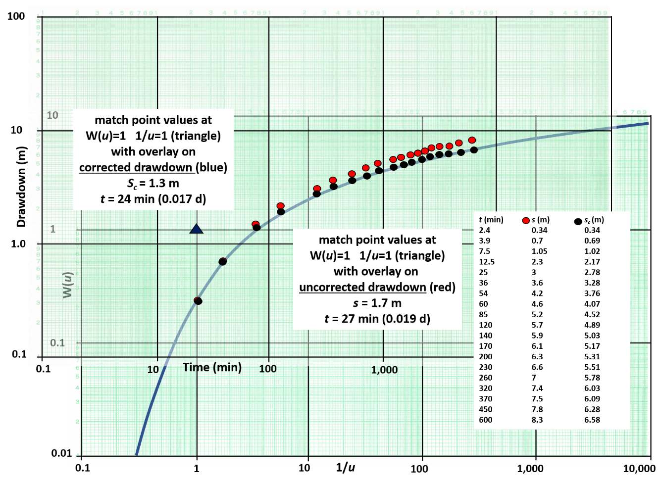
Figure 57 ‑ Unconfined aquifer pumping test data without delayed yield for an observation well located 10 m from a well pumping at a constant rate of 3,000 m3/d. The red dots represent the observed drawdown data. The pre‑pumping saturated thickness was 20 m. The black dots are the corrected data to be used in a Theis curve matching analysis. The black triangle is the match point for the corrected drawdown. The match point location for the uncorrected data is not shown and was derived from a separate curve match (not shown). A table of time‑drawdown data is shown where s is the original field drawdown and sc is the corrected data.
T and Sy are calculated for both the corrected and uncorrected curve matches, so results can be compared. The uncorrected data was matched (not shown) and a match point with values of W(u) = 1, 1/u = 1 (u=1/1=1), s=1.7 m and time = 27 min (0.019 d) was obtained. Using Equations (67) and (68), T and Sy are computed.
[latex]T = \frac{3000\ \frac{m^{3}}{d}}{4\ (3.14)\ 1.7\ m}\ (1) = 140.5\frac{m^{2}}{d}[/latex]
[latex]S_{y} = \frac{1\ (4)\ 140.5\frac{m^{2}}{d}\ 0.019\ d}{{(10\ m)}^{2}} = 0.11[/latex]
Using the match point for the corrected data T and Sy are computed.
[latex]T = \frac{3000\ \frac{m^{3}}{d}}{4\ (3.14)\ 1.3\ m}\ (1) = 183.7\frac{m^{2}}{d}[/latex]
[latex]S_{y} = \frac{1\ (4)\ 183.7\frac{m^{2}}{d}\ 0.019\ d}{{(10\ m)}^{2}} = 0.14[/latex]
The use of the corrected unconfined drawdown results in the hydrogeologic properties of the unconfined aquifer being represented by higher values (not influenced by the effects of dewatering).
This section explains that the Theis solution can be used to represent conditions observed in an unconfined aquifer. When an unconfined system is pumped and little change in saturated thickness occurs, the Theis equation and curve‑matching method can be directly applied. However, when the unconfined system becomes significantly dewatered during pumping T is variable, thus using predicting future drawdown conditions by the Theis method without drawdown correction will overestimate the magnitude of the forecasted drawdowns. The next section presents analytical models used to forecast drawdowns and analyze pumping data sets for unconfined systems that experience delayed yield.