
8.3 Computing T and S from Hydraulic Test Data using the Theis Method
Theis (1935) developed a method to estimate values of T and S from pumping test data. Time and drawdown data are measured in an observation well and then matched to the Theis curve. The method can also be used to compute hydrogeologic properties from time‑drawdown data measured in a pumping well. However, drawdown data require correction when the pumping well is not 100 percent efficient and/or is partially penetrating and/or wellbore storage is significant. These corrections are addressed in the section on using a single pumping well to estimate T and S (Section 12). When drawdown data are collected from one or more observation wells, it is not necessary to correct drawdown for well efficiency because these wells are not pumped so they are effectively 100 percent efficient.
Theis Curve Matching Method
Values of T and S for a fully confined groundwater system can be computed by rearranging Equation (26) to solve for transmissivity as shown in Equation (28). T is directly proportional to the constant pumping rate, Q, and the well function, W(u), and inversely proportional to drawdown.
| [latex]T = \frac{Q}{4\pi s}\ W(u)[/latex] | (28) |
|---|
where:
| T | = | transmissivity (L2T‑1) |
|---|---|---|
| s | = | drawdown (L) |
| Q | = | constant well discharge rate (L3T‑1) |
| W(u) | = | Theis well function (dimensionless) |
The well function is computed for the same time as the drawdown is measured by determining the argument u= r2S/(4Tt). The argument is specific to the radial distance of the observation well from the pumping well and the time at which the drawdown was measured. The equation for u can be rearranged to solve for storativity (S) as shown in Equation (29).
| [latex]S = \frac{u4Tt}{r^{2}}[/latex] | (29) |
|---|
where:
| S | = | storativity (dimensionless) |
|---|---|---|
| u | = | integral argument (dimensionless) |
| T | = | transmissivity (L2T‑1) |
| t | = | time (T) |
| r | = | radial distance to pumping well (L) |
The curve matching technique introduced by Theis (1935) uses the superposition of paper plots to derive match points with values of W(u), 1/u, s and t that are substituted into Equations (28) and (29) to solve for T and S. There is value in understanding how curve matching is performed. The discussions presented in this section and the following sections assume the hydrogeologist will perform curve matching using either hand or computer‑generated log‑log plots of pumping test results, s versus t, and the Theis type curve, W(u) versus 1/u. These curves are physically or electronically superimposed to generate required input for Equations (28) and (29). More recently, curve‑matching software can mathematically generate a best fit of the observation data to the Theis curve. Most programs allow the user to visually examine the best fit and adjust the fit if needed. The use of software to generate estimates of T and S is discussed in Section 13.
The curve matching process involves plotting both the W(u) versus 1/u (Figure 30) and the hydraulic test time‑drawdown (Figure 31) on the exact same size paper using a log‑log scale. Samples of log‑log, semi‑log, and arithmetic paper are provided in Box 1. Curves can also be plotted in a spreadsheet or software program that produces log‑log graphs. All variables increase from the lower lefthand corner of the graphs. A plot of the Theis type curve (Figure 30) is derived by plotting the table of values shown in Figure 26 or generating the plot by substituting values of u into the equation for W(u) (i.e., the term within the brackets of Equation (27)). Some publications (e.g., Lohman 1972) provide paper plots of several different type curves including the Theis type curve. Once again, the field data must be plotted at the same log‑log scale as the type curves.
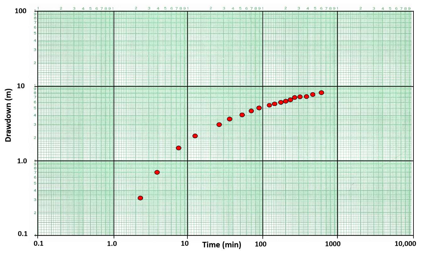
Figure 30 ‑ Hydraulic test drawdown versus time data for an observation well plotted on 3 by 5 cycle log‑log paper at the same scale as the Theis Type Curve in Figure 28. Red dots represent field data collected during a constant rate pumping test.
Once the field data are plotted, the type curve plot is placed on a light table (or glass window) and the field data plot is overlaid (superposed). If computed plots are generated with a spreadsheet program (digital), in software such as Microsoft Excel, test data plots can be modified with a degree of transparency, overlayed and matched to an underlying type curve. It is essential that the log cycles are the same size on the graph paper for the plotted data and the type curve. The field data plot is shifted around keeping the graph axes parallel until a best match of the field data with the type curve is obtained (Figure 31).
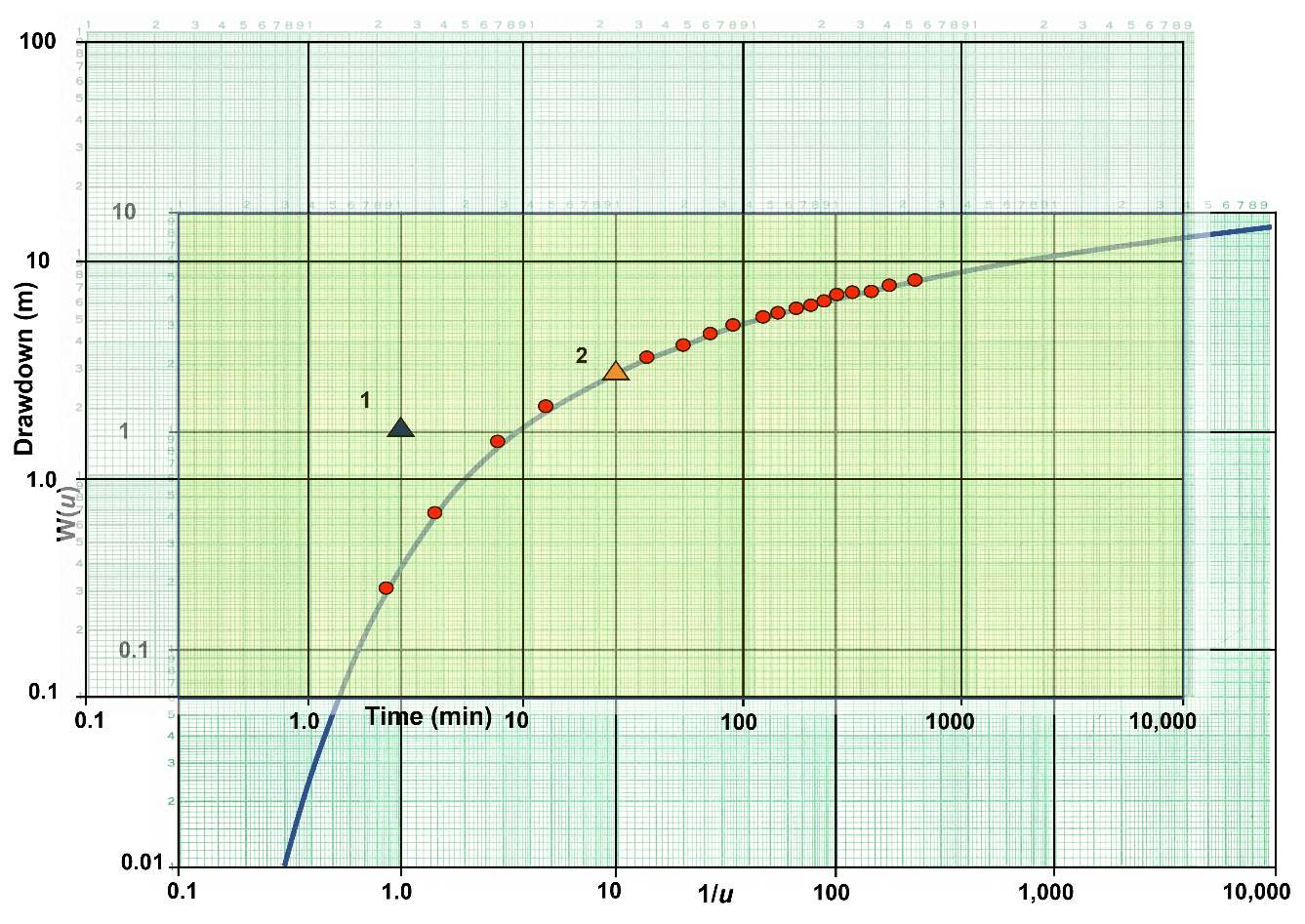
Figure 31 – Example of curve‑matching methodology. Typically, when using a light table, the type curve is laid down and secured then a plot of hydraulic test data (with axes of the same scale as the type curve) is overlain so the data fits on some portion of the type curve. The axes are kept parallel. Once the match is achieved, a match point (triangle) is chosen within the overlapping fields of the graphs (light yellow shaded area). The match point does not have to be on the matched portion of the curve, it can be anywhere within the overlapping field (light yellow). At the match point, values of W(u), 1/u, s, and t are read from the graph axes. Two match points are shown in this example, both will yield equal ratios of the variables. The second match point is not needed but is used in an example calculation to demonstrate that any match point will produce the same results. Match‑point values are then used in Equations (28) and (29) to compute T and S.
Within the overlapping fields of the graphs a single point is chosen to be the match point where values of s, t, W(u) and 1/u are obtained by determining the values of the chosen point on both curves. The match point does not have to be on the portion of the type curve where the data curves were matched. Any match point within the overlapping fields will yield the same ratio of variables (Figure 31). Some investigators use a straight pin to pierce the two sheets of paper at the selected match point site. When doing this the papers can be separated so the data are more easily read from each plot. Once the values at the match point are obtained and the constant pumping rate and radial distance between the pumping well and observation well are inserted in the appropriate equations, Equations (28) and (29), the value of T and S are derived. The computation of S uses the newly computed value of T from Equation (28). The value of 1/u needs to be converted to a value of u. All values used in the calculations must be in the appropriate units so final values of T have dimensions of L2T‑1 and S is dimensionless.
The type curve fitting methodology is a standard methodology used by hydrogeologists to assess drawdown data from a single observation well. This same approach will be used in other sections of this book. A second curve matching procedure can be applied that uses data sets from a single or multiple observation wells. In this case the type curve is plotted as W(u) versus u and one or more observation well data sets are plotted as s verses r2/t on a single graph. The match point selection process is the same as described in the preceding section. This yields values of W(u), u, s, and r2/t. These parameters are then substituted into Equation (28) to compute T and Equation (29) to compute S (where r2/t is converted to 1/(r2/t)). Lohman (1972) illustrates this by using drawdowns from three observation wells on an s versus r2/t log‑log plot, then matching to the type curve and selecting a single match point to compute estimates of T and S.
Example
An example of using pumping test data to derive T and S for a totally confined groundwater system is given here using the data plotted on Figure 30. The test data are collected for an observation well located 200 m from a well pumping at a constant rate of 1.7 m3/min or 2,448 m3/d.
A match point (triangle 1 in Figure 31) is selected within the two over lapping fields. At match point 1 the values of W(u) = 1, 1/u = 1 (u=1/1=1), s=1.7 m and time=2.7 min (0.0019 d). Starting with Equation (28), T is calculated.
[latex]T = \frac{2448\ \frac{m^{3}}{d}}{4\ (3.14)\ 1.7\ m}\ (1)\ = \ 114.6\ \frac{m^{2}}{d}[/latex]
Now with an estimate of T, Equation (29) can be used to compute S.
[latex]S = \ \frac{1\ (4)\ 114.6\ \frac{m^{2}}{d}\ 0.0019\ d}{{(200\ m)}^{2}}\ = 0.000022\ or\ 2.2x10^{- 5}[/latex]
To illustrate that once a curve match has been achieved the location of the match point can be anywhere in the overlapping fields, we calculate T and S from the data at match point 2 on Figure 31. At match point 2, W(u) = 1.8, 1/u =10 (u = 0.1), s =3 m and t =27 min (0.019 d).
[latex]T = \frac{2448\ \frac{m^{3}}{d}}{4\ (3.14)\ 3\ m}\ (1.8)\ = \ 116.9\ \frac{m^{2}}{d}[/latex]
and
[latex]S = \frac{0.1\ (4)\ 116.9\ \frac{m^{2}}{d}\ 0.019\ d}{{(200\ m)}^{2}}\ = 0.000022\ or\ 2.2x10^{- 5}[/latex]
Reading the four values from the graph in Figure 31 at match point 2 produces a small difference in the two computed T values. This is not unexpected as there is some error in reading all four values from the graphs. When match point 1 was selected it was purposely chosen so values of W(u) and 1/u would be clearly defined. Errors reading the s and t values are likely and contribute to the difference in the two T values. The S values are less sensitive to u and t variation and the computed values were within roundoff errors. If the field data curve perfectly matches the type curve, then all T and S values will be identical.
When type curves plotted as W(u) versus u are used with data plots of s versus r2/t, match points will be s, r2/t, W(u) and u. Calculations are undertaken using Equations (28) and (29).
When performing curve matching, in some cases field data may poorly match the type curve for the selected analytical solution. A poor data fit may occur if one or more of the simplifying assumptions used to create the analytical model are violated (e.g., the aquifer is not isotropic and homogeneous), measurement or recording errors are introduced during field data collection, an unrecognized boundary is encountered by the cone of depression, or a constant pumping rate is not maintained. When this occurs, further analysis of the data or application of a different analytical method may be required, otherwise the results are less certain.
Cooper‑Jacob Straight Line Method
Cooper and Jacob (1946) developed a method to analyze confined aquifer pumping tests that involves plotting hydraulic testing results without the need to curve match. Their method approximates the Theis well function, W(u), with the first two components of the infinite series as shown in Equation (30).
| [latex]W(u)\ \cong \ - 0.5772 - \ln\left\{ u \right\}[/latex] | (30) |
|---|
where:
| u | = | r2S/(4Tt) (dimensionless) |
|---|
The Theis Equation is then written with this substitution (Equation (31) or Equation (32)) and referred to as the Cooper‑Jacob approximation (e.g., Freeze & Cherry, 1979).
| [latex]s(r,t) \cong \frac{Q}{4\pi T}\ \ln\left( \frac{Tt}{{1.78r}^{2}S} \right)[/latex] | (31) |
|---|
or
| [latex]s(r,t) \cong \frac{Q}{4\pi T}\ 2.30\ log\left( 2.25\ \frac{Tt}{r^{2}S} \right)[/latex] | (32) |
|---|
where:
| s(r, t) | = | drawdown at distance r and time t (L) |
|---|---|---|
| Q | = | constant pumping rate (L3T‑1) |
| T | = | transmissivity (L2T‑1) |
| t | = | time (T) |
| r | = | radial distance of observation well (L) |
| S | = | storativity (dimensionless) |
| log | = | logarithm base 10 |
| ln | = | natural logarithm |
Because the infinite series is truncated, the solution is only appropriate for values of u < 0.01 or 1/u > 100. When assessing the applicability of the Cooper‑Jacob approximation it is useful to keep in mind that since u = r2S/(4Tt), larger values of T and t and smaller the values of r and S produce smaller values of u. Practically then, drawdown data from observation wells closer to the pumped well and from longer test periods will more likely fit the assumptions of the Jacob method.
Equations (31) and (32) reveal that the drawdown as a function of time in a totally confined aquifer is logarithmic as shown in Figure 30. When field data of drawdown versus time data are plotted as a semi‑logarithmic graph with the drawdown on the arithmetic scale and time on the logarithmic scale, a portion of the curve forms a straight line (Figure 32). The early time and drawdown data are asymptotic to the time axis as the logarithmic scale has no zero point. Cooper and Jacob developed a method that uses the straight‑line portion of the time‑drawdown semi‑logarithmic plot to compute values of T and S.
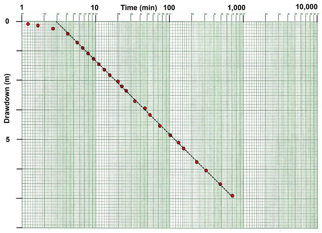
Figure 32 – Example of a semi‑log plot of drawdown and time data (red dots) for an observation well. A straight line (dashed black line) is fitted to the data ignoring the early time data that is asymptotic to the time axis because the log axis has no zero value.
The data presented in Figure 32 can also be plotted with the zero drawdown at the lower left corner. This reverses the slope of the line. The orientation of the y axis (drawdown progression) has no effect on the Cooper‑Jacob methodology.
The T and S values are based on the slope of the straight‑line portion of the curve. Using Equation (32) the slope of the interpreted straight‑line portion of the data is given by Equation (33).
| [latex]s_{2} - s_{1} = \frac{2.3\ Q}{4\pi T}\ \ln\left( \frac{t_{2}}{t_{1}} \right)[/latex] | (33) |
|---|
where:
| s2 | = | drawdown associated with the later time, t2 (L) |
|---|---|---|
| s1 | = | drawdown associated with the early time, t1 (L) |
| Q | = | constant pumping rate (L3T‑1) |
| t2 | = | late time (T) |
| t1 | = | early time (T) |
| T | = | transmissivity (L2T‑1) |
When the time interval equals one log cycle (e.g., log 10 to log 100) then the log of t2/t1 = 1. The change in drawdown for this time interval, s2‑s1 is defined as ∆slog‑t (Figure 33). T is then calculated using Equation (34).
| [latex]T = 2.3\frac{Q}{4\pi{\mathrm{\Delta}s}_{log - t}}[/latex] | (34) |
|---|
where:
| T | = | transmissivity (L2T‑1) |
|---|---|---|
| Q | = | constant pumping rate (L3T‑1) |
| ∆slog‑t | = | change in drawdown over one log cycle of time (L) |
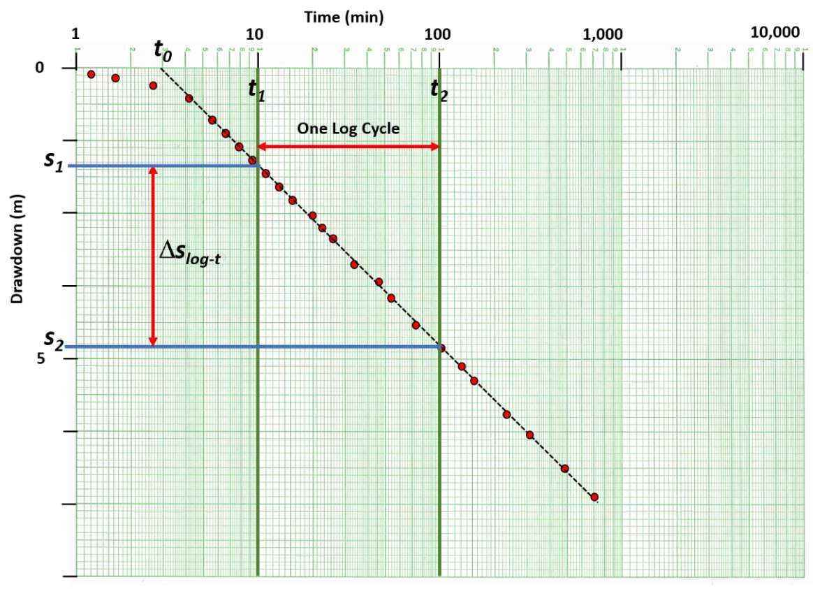
Figure 33 – Semi‑log plot of drawdown (red dots) on an arithmetic scale and time on a log scale collected at an observation well in a confined aquifer. A value of ∆slog‑t is derived as the difference in drawdown (s2‑s1) over one log cycle of time (t1 to t2). The fitted line (dashed black line) is projected to the time axis to obtain a value of t0 where the projected fitted straight line intersects the value of drawdown equal to zero.
The storativity can be estimated using Equation (35) with t0 being the point where the projected fitted straight line intersects the value of drawdown equal to zero (Figure 33).
| [latex]S = 2.25\frac{Tt_{0}}{r^{2}}[/latex] | (35) |
|---|
where:
| S | = | storativity (dimensionless) |
|---|---|---|
| T | = | transmissivity (L2T‑1) |
| t0 | = | time when s = 0 for the fitted straight line (T) |
| r | = | radial distance to the observation point (L) |
The estimate of T using this method is well supported by the mathematical approach. As the slope of the line of field data is smaller (less drawdown measured over time) the value of T is larger. The determination of S using this approach is less robust because small differences in the interpreted slope may result in significant differences in t0 which is based on a logarithmic scale. The use of this method to estimate S is also not recommended when only the pumping well drawdown and time data are available. This is because when the assumptions are not met, for example, the pumping well is not 100 percent efficient and/or is affected by partial penetration effects such that the recorded drawdown is greater than in the adjacent aquifer material. The corresponding interpolated t0 value is then incorrect, yielding incorrect estimates of S. The good news is that when time‑drawdown data are only available from the pumping well, a Cooper‑Jacob plot can be used to approximate T because the slope of the semi‑log plot remains the same whether the well is 100 percent efficient or affected by partial penetration affects (specifics about this are presented in Section 12). It is suggested that the Cooper‑Jacob approximation should only be applied when a semi‑log straight line portion of the drawdown curve dominates the time‑drawdown data, u is small based on estimates of T and S for the unit being pumped, and the Theis model is an appropriate conceptual model for the unit being investigated.
Example
Values of T and S are computed in this example using the data presented in Figure 33. Assuming that the data presented in Figure 33 represent the time‑drawdown data collected 600 m from a well pumping at a constant rate of 2,610 L/min (3,758 m3/d) in a totally confined sand aquifer that is 10 m thick. The change in drawdown over one log cycle of time (10 to 100 min) is: 4.85 m (s2) ‑ 1.32 m (s1) = 3.53 m (∆slog‑t). T is calculated using Equation (34).
[latex]T = 2.3\frac{3758\ \frac{m^{3}}{d}}{4\ (3.14)\ 3.53\ m} = \ 194.9\ \frac{m^{2}}{d}[/latex]
Using the projection of the straight line to the time axis, t0 = 2.8 min (0.0019 d). S is approximated using Equation (35).
[latex]S = 2.25\frac{194.9\ \frac{m^{2}}{d}\ 0.0019\ d}{{(600\ m)}^{2}} = \ 0.000002\ or\ 2x10^{- 6}[/latex]
Cooper‑Jacob Distance‑Drawdown Method
When multiple observation wells are monitored during a pumping test of a confined system, the drawdown data collected at a common time (i.e., t constant) can be used to estimate T and S using the Cooper‑Jacob distance‑drawdown approximation. The idea is that the drawdown data collected simultaneously from at least two wells (three or more is better) located at different radial distances from the pumping well define the character (slope) of the cone of depression (Figure 34). The pumping‑well water level and corresponding radius is not used as a data point because measured drawdown is influenced by well loss and, in some cases, partial penetration (Section 12).
It is logical that when keeping the discharge constant, the steepness and extent of the cone of depression measured in a water‑bearing formation is directly related to the values of T and S (e.g., Figure 29). Shallower cones of depression would be associated with higher values of T and S, whereas lower values would create deeper drawdown cones (pumping rate and other factors held constant). The drawdown collected at two or more observation wells located at different radial distances from the pumping well, s(r1,t), s(r2,t), s(r3,t) and so on (Figure 34) are related to T and S as shown in Equation (36).
| [latex]s(r_{1},\ t)\ - \ s(r_{2},\ t) = \frac{2.3\ Q\ }{2\ \pi\ T}\ \log\left( \frac{r_{2}}{r_{1}} \right)[/latex] | (36) |
|---|
where:
| s(r1,t) | = | the drawdown at distance r1 from the pumping well at time t (L) |
|---|---|---|
| s(r2,t) | = | the drawdown at distance r2 from the pumping well at time t (L) |
| Q | = | constant pumping rate at the production well (L3T‑1) |
| r2 | = | radial distance of observation well 2 (L) |
| r1 | = | radial distance of observation well 1 (L) |
| T | = | transmissivity (L2T‑1) |
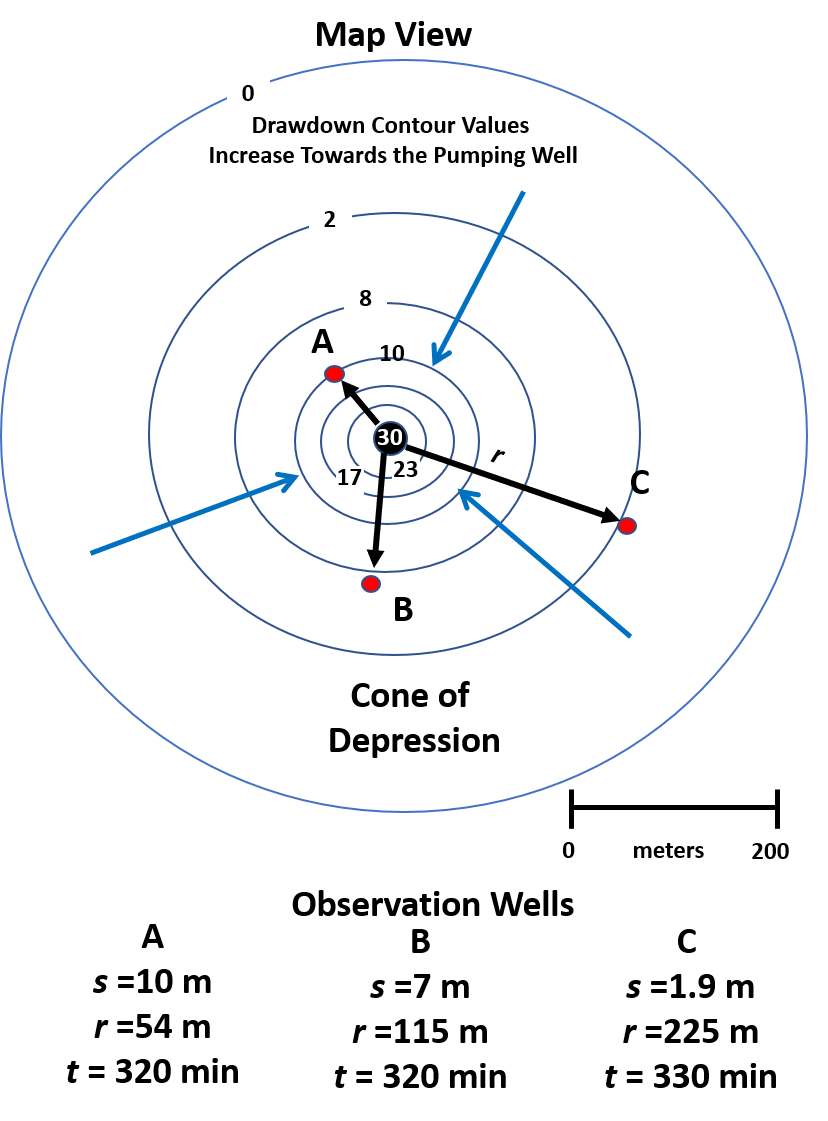
Figure 34 ‑ Schematic map view of the cone of depression in a totally confined aquifer at 320 min after a constant rate of pumping was initiated. Three observations wells (red dots) are located at different radial distances from the pumping well. Blue arrows indicate radial flow to the well. The symbols s, r, and t, indicate drawdown, radial distance, and time since pumping began, respectively.
The transmissivity is determined graphically by computing ∆slog‑r over one log cycle of distance as shown in Figure 35 and applying Equation (37). As was done for the time‑drawdown data, a plot of drawdown at a specified time since pumping started on the arithmetic axis and the observation well radial distances on the log axis is constructed (Figure 35) and estimates of T and S are computed using Equation (37) and Equation (38), respectively. The value for r0 is derived from the location where the fitted straight line crosses the zero‑drawdown axis.
| [latex]T = \frac{2.3\ Q\ }{2\ \pi\ {\mathrm{\Delta}s}_{log - r}}[/latex] | (37) |
|---|
where:
| [latex]S = 2.25\ \frac{Tt}{r_{0}^{2}}[/latex] | (38) |
where:
| S | = | storativity (dimensionless) |
|---|---|---|
| T | = | transmissivity (L2T‑1) |
| r0 | = | radial distance where the fitted straight line crosses s=0 (L) |
| t | = | time (T) |
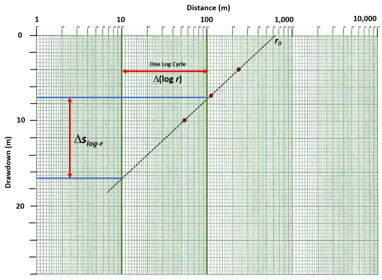
Figure 35 ‑ Plot of the drawdown at a fixed time in the three observation wells shown in Figure 34. The drawdown is plotted on the arithmetic axis and the radial distance from the pumping well to the observation wells on the log axis. A value of ∆slog‑r is derived over a log cycle of r (log (100 m/10 m). Values of T and S are computed using Equations (37) and (38).
Example
Calculating T and S using Equations (37) and (38) is illustrated with the data presented in Figure 34 and Figure 35. Three observation wells provide drawdown data collected 320 min after the production well had been pumping at a constant rate of 3,758 m3/d. The sandstone aquifer is 40 m thick and is totally confined. From the semi‑log plot shown in Figure 35 ∆slog‑r is computed over one log cycle of r.
[latex]\Delta s_{log - r}[/latex] = 16.7 m ‑ 7.4 m = 9.3 m
[latex]T = \frac{2.3\ \left( 3758\frac{m^{3}}{d} \right)\ }{2\ (3.14)\ 9.3\ m}\ \log\left( \frac{100\ m\ }{10\ m}\ \right) = 148\frac{m^{2}}{d}[/latex]
Then, S is approximated using r0 = 640 m.
[latex]S = 2.25\ \frac{148\frac{m^{2}}{d}320\ \min\frac{1\ d}{1440\ \min}}{({640\ m)}^{2}} = 0.00018\ or\ 1.8x10^{- 4}[/latex]
Analyzing Recovery Data
When a pumping well is turned off water levels begins to recover. As shown in Figure 4 the rate of recovery mirrors the drawdown rate. Water levels rise rapidly at first then more slowly at later times. Theis (1935) found that, mathematically, the recovery curve responds as if at the time pumping ceases, the production well continues to pump, but an injection well starts injecting water at the location of the pumping well at the pumping rate. With time the water level fully recovers to near the pre‑pumping level. The final recovery level would theoretically be slightly less than the original static level. This is because a volume of water was removed from storage during the test with no mechanism to replace it. Given an aquifer of infinite extent, this volume is an insignificant portion of the total volume of water in the confined groundwater system, so for practical purposes, the system fully recovers.
The recovery process creates a second set of data for the same test that can be analyzed to estimate T and S. Often observation well recovery data are analyzed and then results compared to the T and S values computed from pumping data. Ideally, they should be identical, but this rarely occurs as differences in curve matching or straight‑line analysis of the data sets introduces some error. Usually, all the hydrogeologic property values derived from drawdown and recovery of observation wells will be averaged to generate values assigned to the water‑bearing unit being tested. Recovery data at the pumping well are often valuable if the pumping well water levels are difficult to monitor because of turbulence in the well casing during pumping or well efficiency effects measured water levels causing them to be lower than theoretical values. When the pumping well is shut off, at early times the water level recovers rapidly, and the frequency of water level data collection should be adjusted to match the drawdown measurement schedule implemented at the beginning of the pumping phase.
When drawdown versus time data from an observation well is plotted on arithmetic scales the difference in water levels during recovery can be described using two terms, residual drawdown, and calculated recovery (Figure 36). The residual drawdown, s’, is obtained by subtracting the observed recovered water level from the corrected‑static water level. The calculated recovery (s‑s’) is obtained by extending the trend of the drawdown curve as if pumping had continued to obtain a projected value of s and subtracting the residual drawdown from that value. Calculated recovery data may include errors because it relies on an accurate estimate of T from the pumping phase of the test which may be in error due to extraneous influences such as variable discharge rate during the pumping phase. In this case the Theis semi‑log method of estimating T is applied.
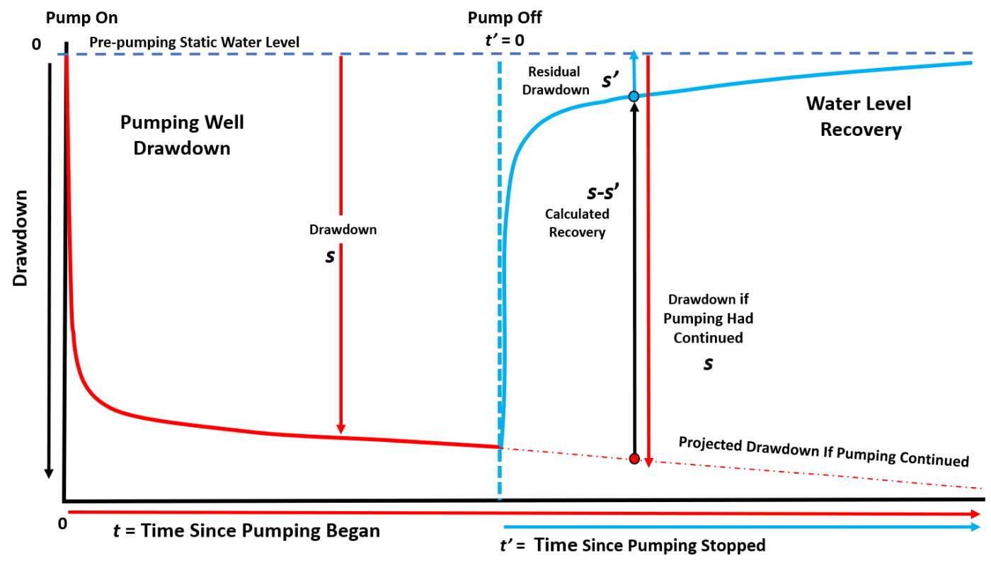
Figure 36 ‑ Schematic of drawdown and recovery data for an observation well is plotted on arithmetic scales. Once the well is shut off the drawdown curve begins to recover at a rate that decreases with time. The remaining drawdown, measured from the corrected‑static water level during recovery, is referred to as residual drawdown, s’. A second description of recovery is provided by the computed calculated recovery, s‑s’. The calculated recovery requires a projection of the drawdown (s) that would occur if the production well was still pumping after the pumping well is shut off. This is represented by the red dash‑dot line that can be projected from the drawdown rates observed at the time the pump was shut off or calculated once the aquifer parameters have been estimated from the drawdown portion of the data set.
Theis Semi‑log Method for Estimating T from Residual Recovery Data
Theis (1935) presented a procedure to estimate T that eliminates the complications of estimating residual recovery from a projected drawdown curve by using the residual drawdown data directly. In this case, the residual drawdown s’ is plotted versus t/t’ on a semi‑log plot as shown in Figure 37. [latex]\Delta s_{log - t}'[/latex] is derived over one log cycle of t/t’ where t is the time since the pumping started and t’ is the time since the pump was shut off. T is calculated using Equation (39).
| [latex]T = 2.3\frac{Q}{4\pi\Delta s_{log - t}'}[/latex] | (39) |
|---|
where:
| T | = | transmissivity (L2T‑1) |
|---|---|---|
| Q | = | constant pumping rate (L3T‑1) |
| [latex]\Delta s_{log - t}'[/latex] | = | the change in residual drawdown over one log cycle change t/t’ (L) |
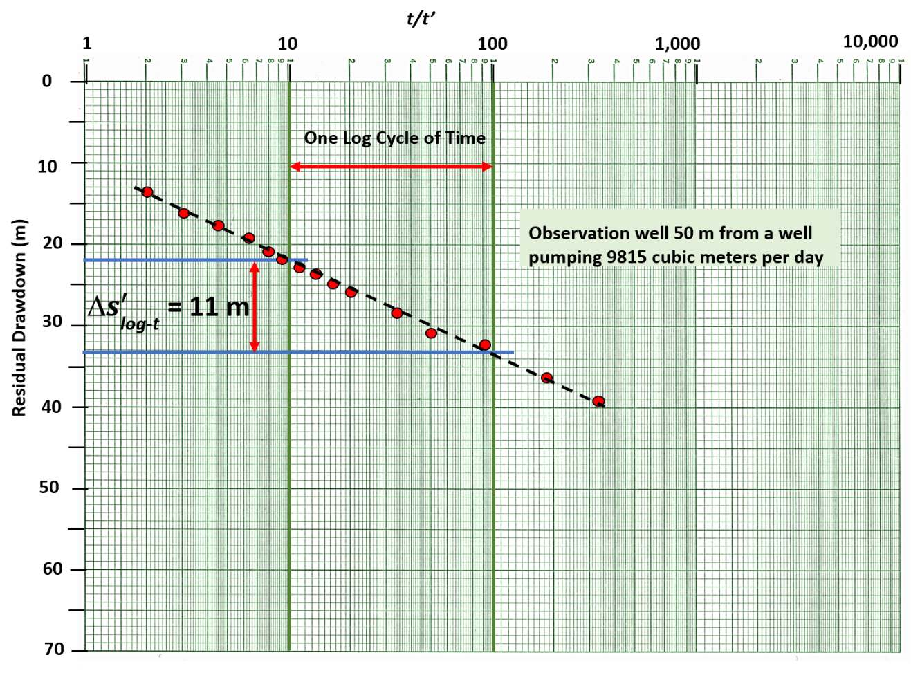
Figure 37 ‑ Semi‑log plot of residual drawdown versus t/t’ in an observation well 50 m from the pumping well, The time since the pumping started is t and the time since the pumping stopped is t’. The slope of the projected straight line (dashed black line) is determined to be 11 m over one log cycle of t/t’.
This methodology is not used to derive a value of S. Kruseman and de Ridder (2000) provide further explanation of how residual drawdown data are used. Their textbook is supplied without cost on the gw‑project.org website.
Example
Using the data presented in Figure 37 along with the information that the well was pumped at a constant rate of 9,815 m3/d for 100 min. The graph reveals that [latex]\Delta s_{log - t}'[/latex]is 11 m.
[latex]T = 2.3\frac{Q}{4\pi\Delta s_{log - t}'} = 2.3\frac{9815\ \frac{m^{3}}{d}}{4\ (3.14)\ 11\ m} = 163\frac{m^{2}}{d}[/latex]
Theis Curve Matching Method for Estimating T using Calculated Recovery Data
Calculated recovery data can be used to estimate T and S but provides less certain results because variation in pumping rate may lead to an inaccurate projected drawdown curve that us used to calculate recovery. For this analysis, calculated recovery is plotted versus time since pumping stopped—setting time zero at the time the pump was turned off—as illustrated in Figure 36. Calculation of T and S is described by Sterrett (2007). The calculated recovery s‑s’ versus t’ is plotted on a log‑log scale (Figure 38) and matched to the Theis type curve plotted at the same scale to derive the four match point values: s‑s’, t’, W(u) and 1/u. These are used in Equations (40) and (41)—which are modifications of Equations (28) and (29)—to calculate T and S, respectively. The match point is shown in Figure 39. The projected drawdown after pumping ceases can be in error because it is estimated, and this may cause error in the estimated T and S values.
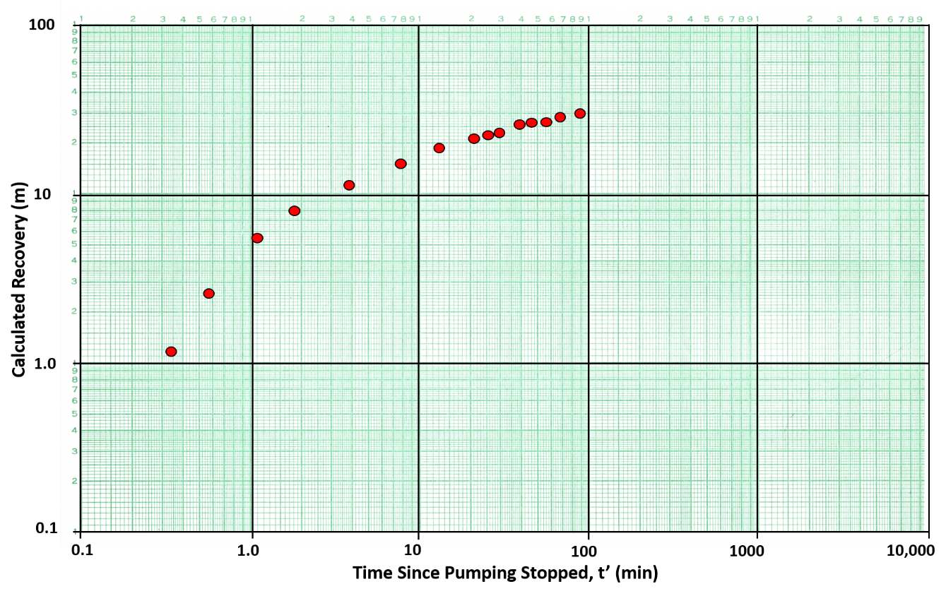
Figure 38 ‑ Plot of calculated recovery versus time since the pumping stopped on log‑log scales for water levels in an observation well that is 65 m from the pumping well. Red dots are calculated recovery values.
| [latex]T = \frac{Q}{4\pi\left( s - s' \right)}\ W(u)[/latex] | (40) | |
|---|---|---|
| [latex]S = \frac{u4Tt'}{r^{2}}[/latex] | (41) |
where:
| T | = | transmissivity (L2T‑1) |
|---|---|---|
| Q | = | constant pumping rate (L3T‑1) |
| s‑s’ | = | calculated recovery (L) |
| W(u) | = | Theis well function (dimensionless) |
| S | = | storativity (dimensionless) |
| u | = | integral argument (dimensionless) |
| t’ | = | time since the pumping stopped (T) |
| r | = | radial distance to pumping well (L) |
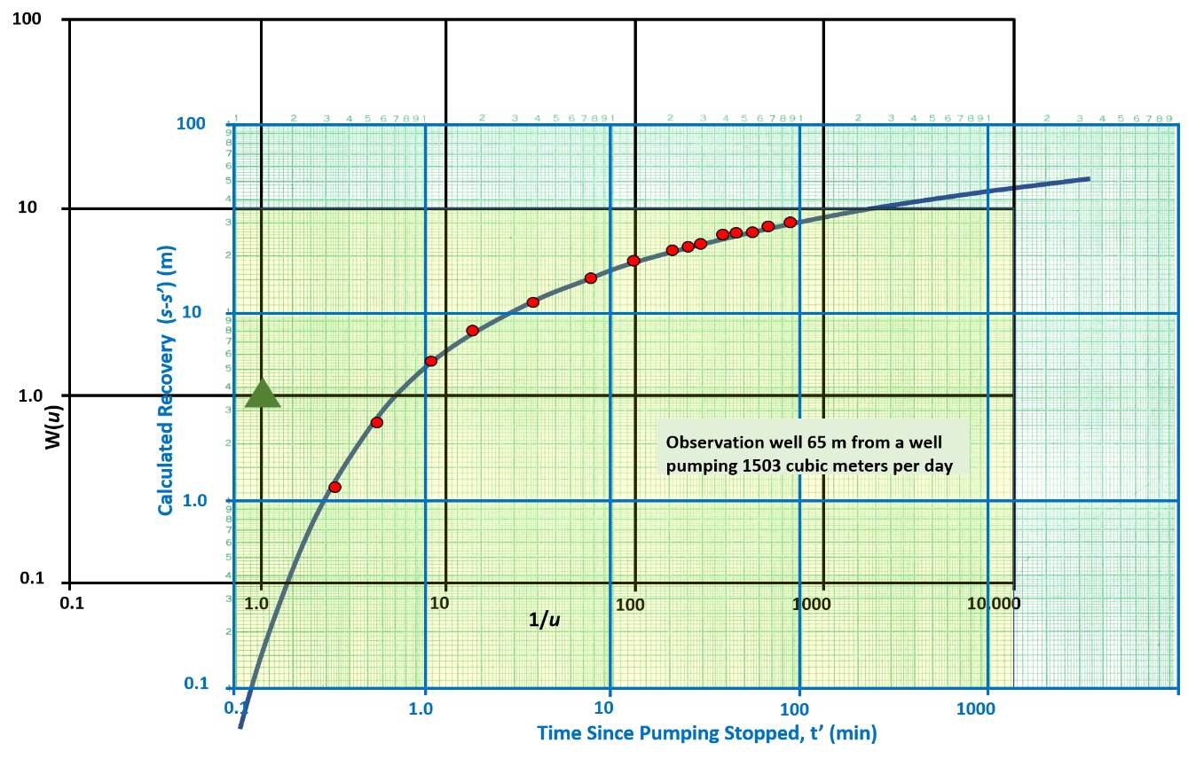
Figure 39 ‑ Curve match for calculated recovery versus time and the Theis curve. Match point is W(u)=1, 1/u=1, calculated recovery (s‑s’)=3.6 m, and t’=1.3 minutes.
Example
Using Equation (40) and information that the pumping well yielded 1,503 m3/d and the observation well was 65 m from the pumping well; along with the data in Figure 38, values of T and S can be calculated using recovery data. From Figure 38, W(u) = 1, 1/u = 1, calculated recovery (s‑s’) = 3.6 m, and t’ = 1.3 min.
[latex]\ T = \frac{Q}{4\pi\left( s - s' \right)}\ W(u)\ = \frac{1503\ \frac{m^{3}}{d}}{4\ (3.14)\ (3.6\ m)}(1)\ = \ 33.2\frac{m^{2}}{d}[/latex]
Using Equation (41), an estimate of S can be derived as shown here.
[latex]S = \frac{u4Tt'}{r^{2}} = \frac{(1)\ (4)\ 33.2\ \frac{m^{2}}{d}1.3\ \min\frac{1\ d}{1440\ min}}{{(65\ m)}^{2}} = \ 0.000028\ or\ 3x10^{- 5}[/latex]
Variable Discharge Pumping Test
The application of most analytical solutions to pumping test data require the pumping discharge be held at a constant rate during the test. If the rate varies significantly during a test, typically a weighted average pumping rate is computed. This is accomplished by assigning a pumping time interval for each measured discharge, multiplying each discharge variation by the interval time, adding these time‑weighted discharge intervals together and dividing by the total pumping time. An example is provided in Section 5.4.2. Ideally, when a constant discharge test is planned, variations in discharge will be small.
Evaluation of tests with significant variability in discharge rates is beyond the scope of this book. The US Department of Energy provides an open‑source software package that can be used for such advanced analyses called nSIGHTS↗ (n‑dimensional Statistical Inverse Graphical Hydraulic Test Simulator). The department provides an overview of the software application↗ in the form of a PowerPoint presentation.
Lohman (1972) presents an additional straight‑line solution for a fully confined aquifer where the drawdown is constant and the pumping‑well discharge is allowed to vary over time. All other Theis assumptions are applicable. This condition is most commonly associated with conducting a pumping test using a flowing well that is fully opened from its static state at the beginning of the test. Jacob and Lohman (1952) derived equations and solution methods for this condition. The reader is referred to Lohman (1972) for details of the mathematical derivation and application of the methodology.
Applicability Of Methods Presented in this Section
Each of the methods used to process and analyze pumping test data described in this section apply to totally confined systems. However, Theis’s curve‑matching methodology is not restricted to analyzing test results from a fully confined system. This technique is used to analyze the response of leaky, and unconfined systems by using early‑time drawdown data. In the early portion of the pumping test, the drawdown closely matches the Theis function as shown in Figure 40, so aquifer properties can be estimated by matching that portion of the data to the Theis well function. The log‑log plots of drawdown are also used to assess whether boundaries may be influencing observed drawdown (Figure 40). Experienced hydrogeologists review the shape of a log‑log plot of test data and use that information to assist them in selecting an appropriate analytical approach.
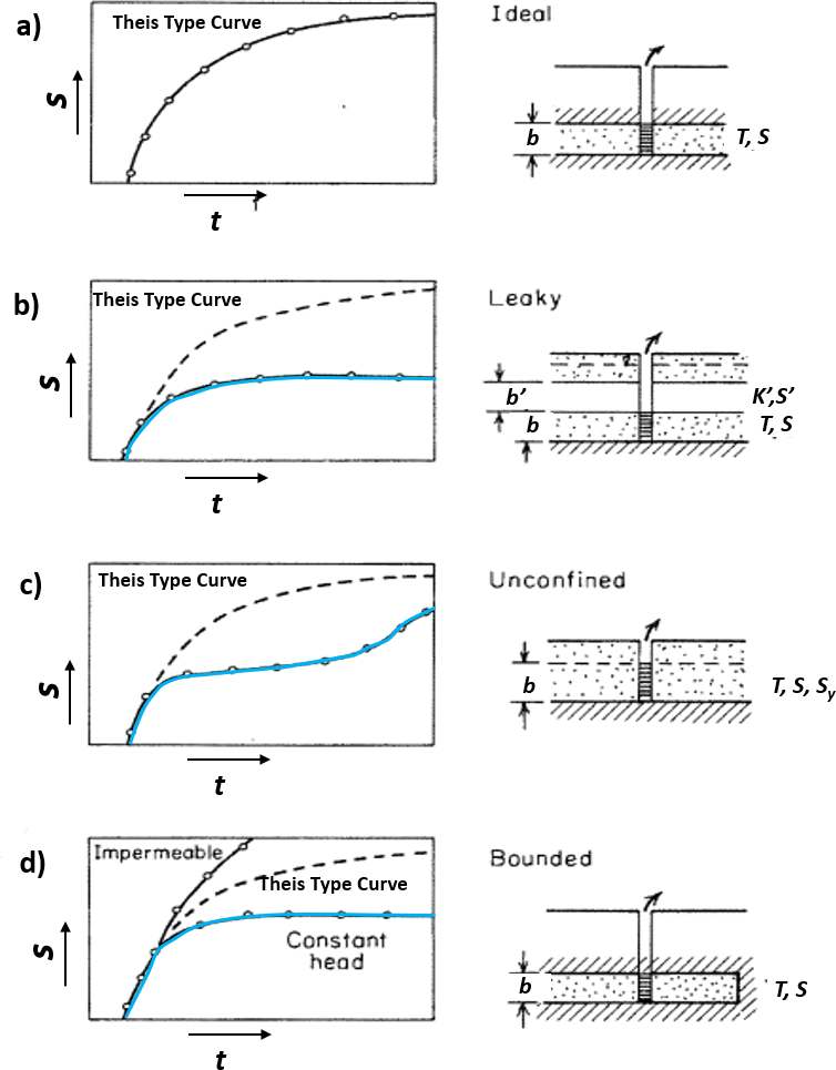
Figure 40 ‑ Schematics of log‑log plots of time (x axis) and drawdown in an observation well (y axis) showing ideal drawdown behavior in response to a constant discharge pumping test of an isotropic and homogeneous groundwater unit (speckled unit). T is transmissivity, S is storativity, Sy is specific yield, b is the initial saturated thickness of the unit, b’ is the thickness of a leaky confining unit, K’ is the vertical hydraulic conductivity of the leaky confining unit, and S’ is the storativity of the confining unit (modified from Freeze & Cherry, 1979).
a) Pumping response to ideal Theis conditions. Pumping test data (open circles) fall on the curve. The dashed line in illustrations b‑d is the ideal Theis response (a totally confined system) that is used for comparison.
b) Pumping response to leakage through the leaky confining unit (blue line open circles). In this setting, data fall below the Theis curve and reach equilibrium.
c) Pumping response to unconfined conditions (open circles). The data match the Theis response at early times then drawdown slows (blue line) due to drainage of water from pores at the water table. Drawdown may reach an equilibrium and then increase to join the Theis curve trend at later times.
d) Pumping response when lateral boundaries are encountered, a lateral recharge boundary (blue line) where drawdown is constant after inflow equals well discharge and a lateral impermeable boundary (solid black line) where drawdown is larger than the Theis curve.
Section 9 discusses how pumping‑test time‑drawdown data for a confined system are affected by the addition of water from overlying or underling confining units and aquifers during testing.