
11.1 Well Interference
Well interference occurs when the cone of depression of two or more pumping wells overlap (Figure 66). As a well is pumped its cone of depression expands over time. If a second well in the same aquifer is also pumping its cone of depression also expands. In the regions of the aquifer where the cones of depression overlap, the drawdown in the zone of overlap is the composite drawdown from both pumping wells. Drawdown at a location affected by multiple pumping wells is additive in linear systems (e.g., fully confined aquifers with laminar flow). Additive means that the solutions can be calculated separately and superposed (i.e., added together). Where the linearity is not applicable (e.g., unconfined aquifers with more than about 10 percent drawdown, dewatering of confined aquifers, turbulent flow in open fractures) then superposition may not be valid and should be used with caution. The more nonlinear the conditions the greater the error in the superposed solution.
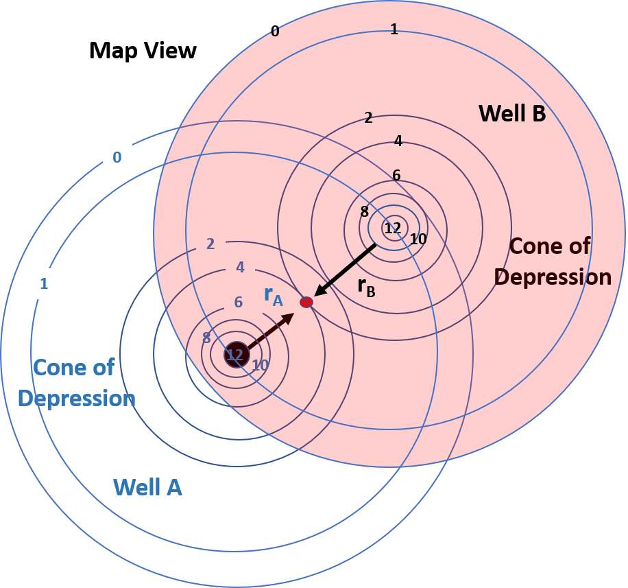
Figure 66 ‑ Illustration of well interference created by pumping two wells at the same rate for an equal length of time. The wells penetrate a totally confined aquifer that is isotropic and homogeneous. Both wells A and B are constructed similarly, and their pumping rate and schedule is the same in this example. The pumping wells could each operate at any rate for any length of time and the approach to generating a composite cone of depression is the same. The red dot represents the location of an observation well that is not pumping. The schematic shows drawdown for each well as contours in units of length. rA and rB are the radial distances to the unpumped observation well from wells A and B.
The term well interference is used when a pumping well is influenced by drawdown from one or more nearby pumping wells. At the observation well location (red dot, Figure 66) the overlapping cones of depression show that at this time the observation well is experiencing a drawdown of 4 units from pumping of Well A and 2 units from pumping of Well B. The total drawdown at the observation well under the confined conditions is 6 units. The pumping of both wells also affects the drawdown in the pumping wells. Both pumping wells create a drawdown of 12 units at the pumping well location and experience an additional drawdown of 1 unit from the other pumping well for a total of 13 units of drawdown in both pumping wells. A sketch of the composite cone of depression is shown in Figure 67.
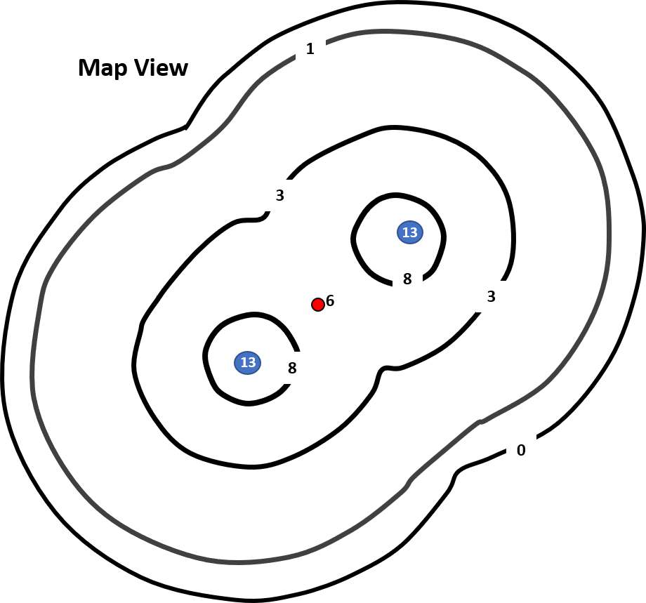
Figure 67 ‑ Sketch of the composite cone of depression created from conditions illustrated in Figure 66. This diagram was created by assigning combined drawdowns to locations where the drawdown contours overlapped and then hand contouring the resulting drawdown values. The blue dots are the pumping wells where the composite drawdown is 13 units of length. The red dot represents an observation well drawdown of 6 units of length. The black lines represent contours of drawdown in units of length.
Figure 67 shows the resulting cone of depression due to well interference in map view. Well interference can also be viewed in cross section (Figure 68). The same approach can be used to determine the interference effect of multiple wells pumping at different rates and for different lengths of time on any pumping or observation well located in the zone of interference. Combining the drawdowns by adding the effects at a location is referred to superposing the cones of depression and the method is referred to as superposition. In well fields where multiple wells are pumping on different schedules and at different rates the resulting potentiometric surface reflects well interference (composite water levels) as shown in Figure 69.
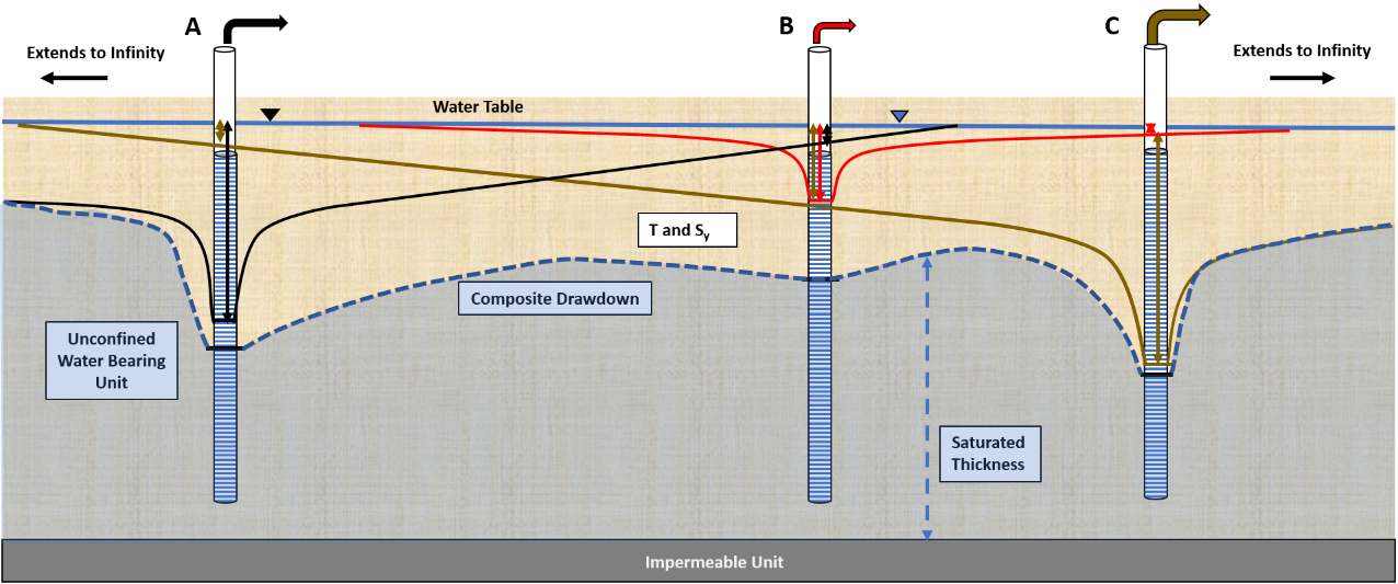
Figure 68 ‑ Schematic cross section showing well interference and the resulting drawdown profile for an isotropic and homogeneous unconfined aquifer effected by pumping of three wells. The drawdown at each well is shown by arrows keyed to the color of the well discharge (Well A black, Well B red, Well C brown). When the well drawdown profiles are superimposed, the drawdowns are added, and the composite drawdown profile is obtained (dashed blue line). Determining well interference in an unconfined aquifer is more difficult than in a confined aquifer because transmissivity decreases as drawdown increases increasing the drawdown relative to that in an aquifer of constant saturated thickness.
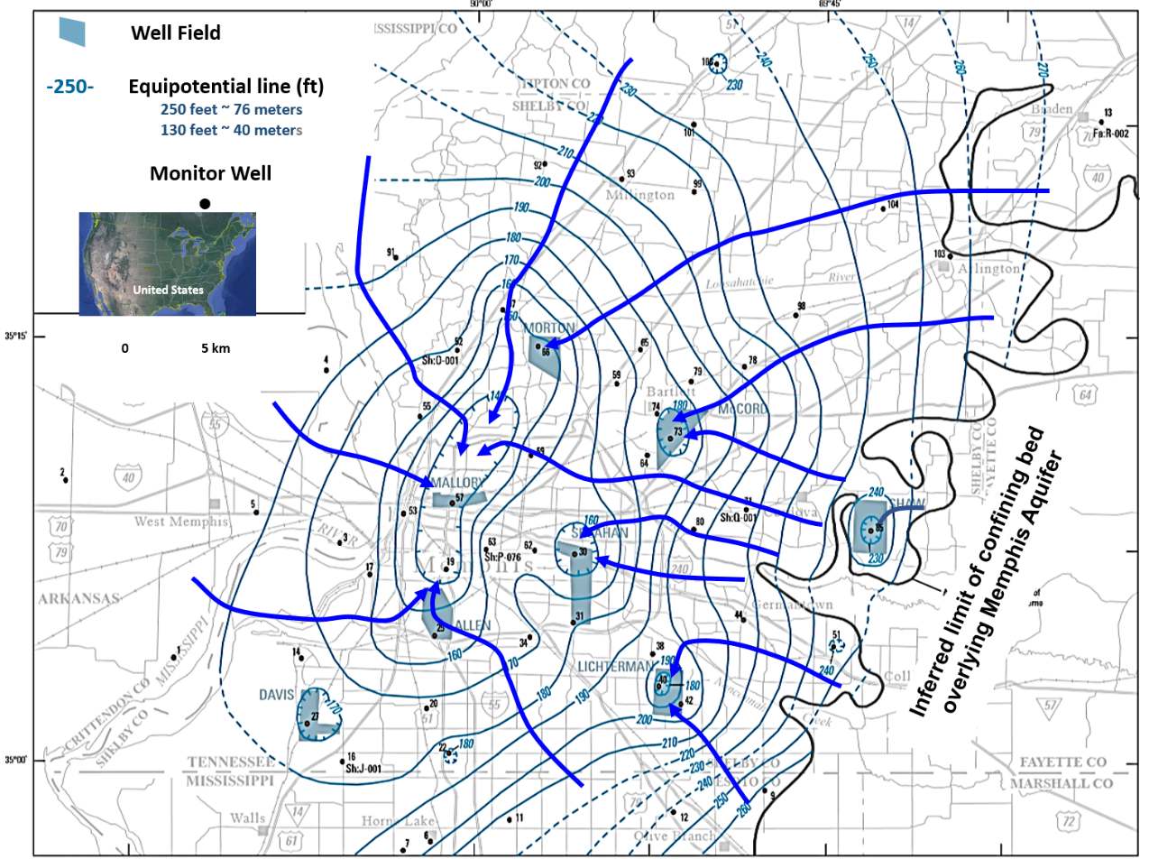
Figure 69 ‑ Potentiometric surface based on September to November 2010 water level data for the confined Memphis Sand Aquifer located beneath Memphis, Tennessee, USA. Equipotential lines are solid green and dashed where inferred. All units are in feet. Hatched contours indicate depressed areas of the potentiometric surface associated with pumping centers (well fields) that have operated for an extended period of time. The curved black solid line in the eastern portion of the area represents the location of the transition from unconfined conditions in the east to confined conditions in the west. Flow lines are blue arrows. Pumping has captured groundwater flowing throughout the area as flow lines converge at well field locations where multiple wells are pumping. Initial groundwater flow was from southeast to the west, now production wells have altered the flow paths with groundwater principally moving to the pumping centers (lowest potentiometric contours) (modified from Kingsbury, 2018; Woessner & Poeter, 2020).
This superposition methodology is straightforward and can be used to remove unwanted interference that occurs during a hydraulic test (a single well pumping at a constant rate) affected by unplanned starts and shutdowns of other nearby pumping wells. This is shown in Figure 70 where startup and shut down of two adjacent pumping wells effect drawdown at a pumping test observation well. Such effects need to be removed before analyzing the data to estimate values of T and S.
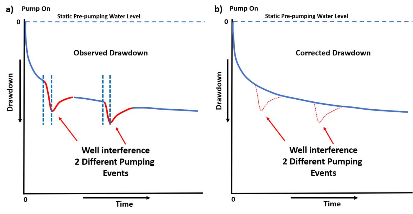
Figure 70 ‑ Arithmetic plots of observed drawdown in a pumping test observation well. a) Drawdown where nearby wells start up and shut down (vertical dashed blue lines) during the test. The red portions of the drawdown curve represent the composite drawdown at the observation well and interference from the adjacent pumping wells. b) Pumping drawdown data are corrected for the well interference by removing the additional drawdown from the adjacent pumping wells and reproducing the drawdown trend (solid blue line).
In some settings, the startup and shut down of additional pumping wells may not affect pumping or observation well drawdown because they are located too far from the test well or pumping rates and durations are too small to cause identifiable interference. When estimates of the tested formation T and S are known, the degree of interference from other pumping wells can be computed from standard well hydraulic equations before initiation of a pumping test (e.g., Theis equation; Hantush‑Jacob equation, etc.).