
10.3 Formulating Delayed Yield Analysis
Section 6 stated that differential equations describing the response of drawdown to pumping in unconfined settings are non‑linear and cannot be solved directly because the independent variables (e.g., thickness and transmissivity) are a function of the dependent variable (i.e., head). Analytical approaches describing the response of unconfined groundwater systems have been developed assuming transient drawdown behavior can be approximated by combinations of linear differential equations. Analytical equations developed to represent the delayed yield process are mathematically complex and different representations of the delayed yield analytical solutions yield slightly different values of aquifer properties (e.g., Lin et al., 2019; Nwankwor et al., 1992).
As described in Lohman (1972), Boulton (1954a, 1954b, 1963) along with Boulton and others (1964) developed a set of analytical equations and type curves to analyze hydraulic testing data exhibiting delayed yield. These approaches were modified by Neuman (1972, 1974, 1975). He generated a linear differential equation that assumed a line sink for the pumping well and instantaneous drainage from the capillary fringe and unsaturated zone above the water table (Moench et al., 2001).
Strictly speaking, it is not correct to assume “instantaneous release of stored water from pores at the water table”. Drainage occurs from pores within the capillary fringe and unsaturated pores above the capillary fringe but this drainage is not instantaneous. As the water table declines, a vertical hydraulic gradient occurs within the zone above the water table including the capillary fringe, especially near the pumped well (Nwankor et al, 1992). Drawdown of the capillary fringe is slower than drawdown of the water table. For this reason, it is best to use drawdown data from observation wells that are several aquifer thicknesses distant from the pumped well where vertical gradients within the saturated zone are very small.
Since Neuman’s work a number of authors have attempted to incorporate the effect of the release and movement of water in the capillary fringe and unsaturated zone within the cone of depression into delayed yield analytical solutions (e.g., Moench et al, 2001; Nwankwor et al., 1992). Lin and others (2019) provide a good summary of previous efforts and a modified method to assess unconfined hydraulic tests with delayed yield. The equations they derived are solved and linked with field test data using sophisticated numerical methods. Methods developed by Tartakovsky & Neuman (2007) and Moench (1997) are available most commercial software packages (Section 13).
Neuman’s curve matching methods are presented here to be consistent with other sections of this book. Moench and others (2001) state that for the conditions they evaluated, Neuman curve matching with late time data provided reasonable estimates of T, Kh, Kz, and Sy (where Kz is the vertical hydraulic conductivity of the aquifer). However, their work and the work of others revealed that Neuman’s approach missed the effects of storage‑release processes at early times. They argue that other methods to estimate storage properties should be used when relying on early and intermediate drawdowns. Such methods account for the addition of stored water to the water table by unsaturated flow processes (Moench et al., 2001).
Recognizing these issues, this book presents the curve‑matching method described by Neuman (1975) which is found in many groundwater textbooks. It provides tables of variables and plotted families of curves. Readers interested in a more detailed discussion of delayed yield representations will find it in Moench and others (2001) and Lin and others (2019). Commercial software packages typically include the Neuman method as well as other methods that can be used to analyze unconfined pumping test results. Lists of software and the methods they employ are provided in Section 13 of this book.
Mathematical Development of a Delayed Yield Analysis Method
The Neuman (1974, 1975) solution involves an integral with three variables, ua, uy, and η as shown in Equation (70). W(ua,uy,η) is the Neuman well function. Schwartz and Zhang, (2003) note that evaluation of Neuman’s analytical solution takes “…a large amount of time”. Strengthening his original work, numerical methods have been applied to increase accuracy and efficiency of computations (Moench & Qgata, 1984; Moench 1993, 1995, 1996). The resulting general equation is described by Equations (70), (71), (72), and (73).
| [latex]s(r,t) = \frac{Q}{4\pi T}\ W\left( u_{a},u_{y,}\eta \right)[/latex] | (70) | |
|---|---|---|
| [latex]u_{a} = \frac{r^{2}S}{4Tt}[/latex] | (71) | |
| [latex]u_{y} = \frac{r^{2}S_{y}}{4Tt}[/latex] | (72) | |
| [latex]\eta = \frac{r^{2}K_{z}}{b^{2}K_{h}}[/latex] | (73) |
where:
| s(r,t) | = | drawdown at a radial distance r and time t (L) |
|---|---|---|
| Q | = | constant well discharge rate (L3T‑1) |
| T | = | transmissivity (L2T‑1) |
| S | = | storativity under early time confined conditions (bSs) (dimensionless) |
| b | = | pre‑pumping saturated thickness (L) |
| Ss | = | specific storage (L‑1) |
| Sy | = | storativity at late times, specific yield (dimensionless) |
| t | = | time (T) |
| r | = | radial distance to the observation well (L) |
| W (ua,uy,η) | = | Neuman unconfined well function (dimensionless) |
| ua | = | early time values of u (dimensionless) |
| uy | = | late time values of u (dimensionless) |
| Kz | = | unconfined vertical hydraulic conductivity (LT‑1) |
| Kh | = | unconfined horizontal hydraulic conductivity (LT‑1) |
Computation of drawdown at an observation well located some distance r from the pumping well requires values of T, S, and Sy, the initial saturated thickness of the aquifer b, and the horizontal and vertical hydraulic conductivity values of the unconfined aquifer as indicated in Equations (70) through (73). These parameters are used to generate a value of the well function, W(ua,uy,η), from compiled tables (Figure 60 and Figure 61). Computations to predict drawdown using Equation (70) can then be made for any value or r and t. Early time drawdown prediction uses ua of Equation (71) and late time drawdown prediction uses uy of Equation (72).
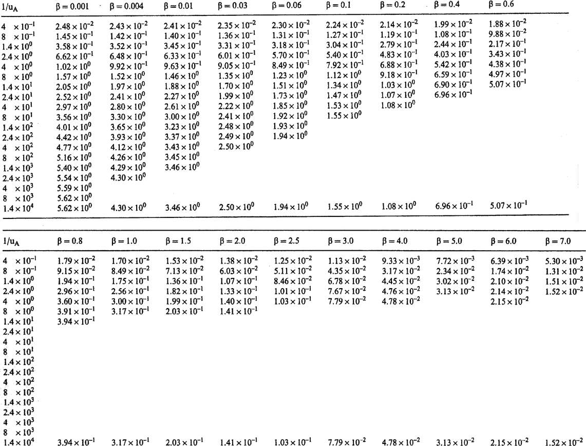
Figure 60 ‑ Table of well function values for early times presented by Kruseman and de Ridder (2000) for the Neuman well function for unconfined aquifers with delayed yield. They used a slightly different notation than presented in this book, using uA as equivalent to ua and β in the place of η. That is, values of β in this table are equivalent to η in this book (after Kruseman & de Ridder, 2000).
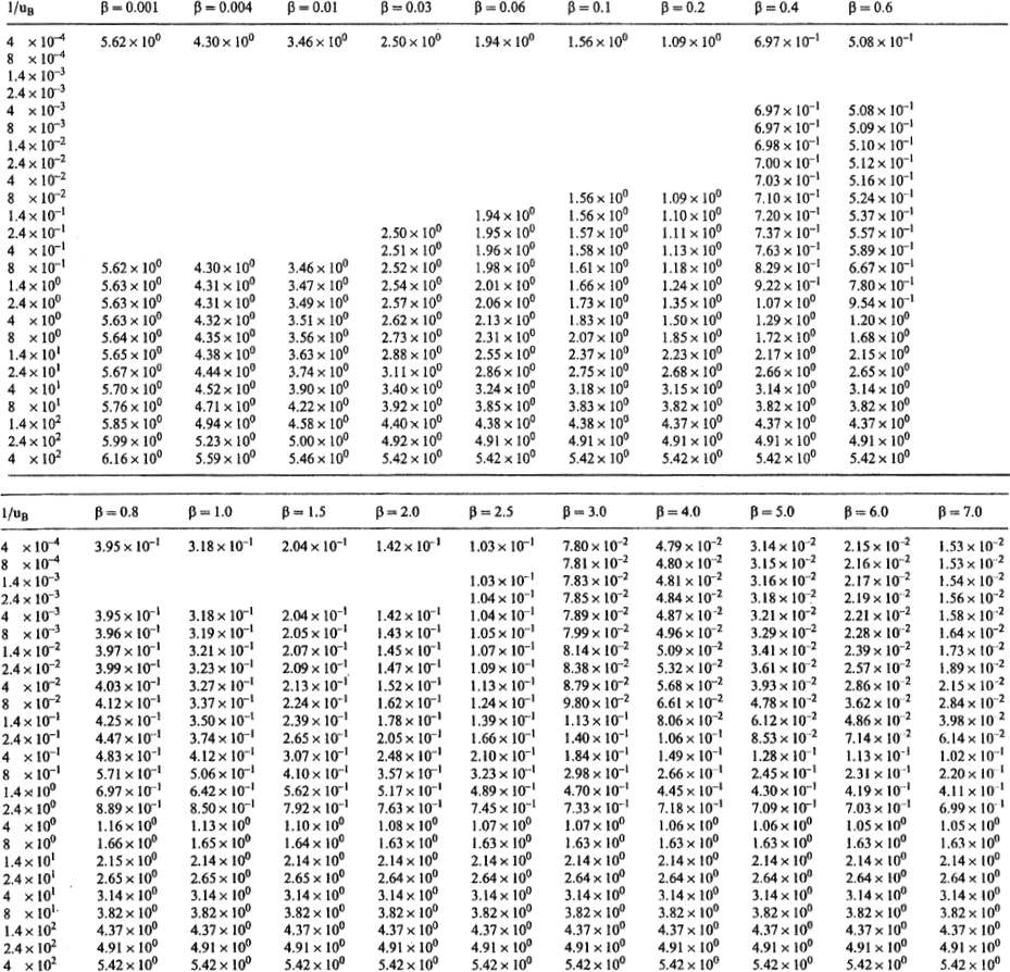
Figure 61 ‑ Table of well function values for late time presented by Kruseman and de Ridder (2000) for the Neuman well function for unconfined aquifers with delayed yield. They used a slightly different notation than presented in this book, using uB as equivalent to uy and β in the place of η. That is, values of β in this table are equivalent to η in this book (after Kruseman & de Ridder, 2000).
As stated previously, the table of values (Figure 60 and Figure 61) represent a subset of values that are generated by substituting combinations of ua, uy , and η into the analytical solution to produce values of W(ua,uy,η). The values in the tables can be plotted to create type curves. If type curves with other values of η are required they can be generated using an available analytical solution (e.g., Neuman, 1972, 1974, 1975). Most often other values of η are interpolated from the tables shown in Figure 60 and Figure 61.
Example
In this example the drawdown at an observation well located 200 m from the pumping well in an unconfined aquifer is computed. The pre‑pumping saturated thickness is 30 m, T = 3,000 m2/d, Sy = 0.15, Kz = 10 m/d and Kh = 100 m/d. Assume the well has been pumping at a constant rate of 2,505 m3/d for 1 day and that delayed yield is likely to have ceased. The late time uy value is used to estimate storativity.
[latex]u_{y} = \frac{(200\ \text{m})^{2} 0.15}{4\left(3000\frac{\text{m}^{2}}{\text{d}}\right)(1\ \text{d})} = 0.5,\ \text{then}\ \frac{1}{u_{y}} = 2 = \frac{1}{u_{B}}\ \text{of Figure 61}[/latex]
[latex]\eta = \frac{(200\ \text{m})^{2}\ 10\frac{\text{m}}{\text{d}}}{(30\ \text{m})^{2}\ 100\frac{\text{m}}{\text{d}}} = 4.4 = \beta\ \text{of Figure 61}[/latex]
The following values are from Figure 61.
| 1/uB equivalent to 1/uy of this book | β equivalent to η of this book | W(uA,uB,β) equivalent to W(ua,uy,η) of this book |
|---|---|---|
| 1.4 | 4.0 | 0.455 |
| 2.4 | 4.0 | 0.718 |
| 1.4 | 5.0 | 0.430 |
| 2.4 | 5.0 | 0.709 |
Using the values from Figure 61 and linear interpolation, first estimate the value of the well function associated with β=4 and 1/uB=2, which is W(uA,uB,β)=0.6128. Next determine the well function value associated with β=5 and 1/uB=2, which is W(uA,uB,β)=0.5974. Finally, interpolate between those values for the well function associated with 1/uB=2 and β=4.4, which is W(uA,uB,β)=0.6066. Then, substituting these values into Equation (70), knowing that for uy=0.5, 1/uB=2, η=4.4, and W(ua,uy,η)=0.6066, s=0.04 m as show here.
[latex]s = \frac{2505\frac{m^{3}}{d}}{4\ (3.14)\ 3000\frac{m^{2}}{d}}\ (0.6066) = 0.04\ m[/latex]