
Box 9 Laboratory Methods used to Determine Hydraulic Properties of Aquitards and Low Permeability Formations
Small samples of aquitard and low permeability formations can be examined in the laboratory and estimates of the hydraulic conductivity and specific storage derived. Some transient field‑scale testing results are stated in terms of diffusivity, Kh/Ss and Kv/Ss. Thus, measurements of specific storage are of value because they can be used to solve for hydraulic conductivity in transient settings.
As with any laboratory testing it is assumed that the sample is representative of the material under investigation. As previously mentioned, laboratory methods may appropriately represent field conditions when the confining unit is uniform and coarse‑grained lenses or secondary permeability features are not present.
Methods discussed in this box include the falling head permeameter, triaxial cell, and consolidometer.
Box 9.1 Falling Head Permeameter (modified from Box 4.3 of Woessner and Poeter (2020)
The falling head permeameter was designed to determine hydraulic conductivity values of low permeability sediments. In this method the water levels and flow rates change over time. Data requirements include the dimensions of the sample and connected tube, and the change in water level over time as shown in Figure Box 9‑1.
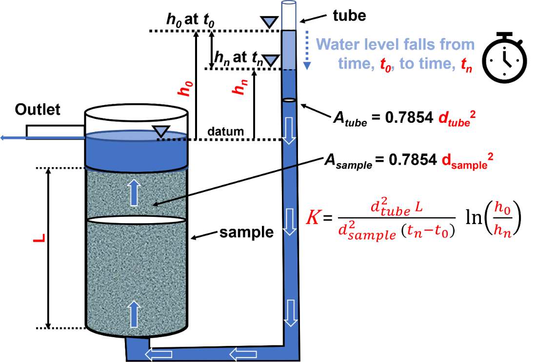
Figure Box 9‑1 ‑ Schematic of a falling head permeameter. The sample of length L is placed in a chamber of area [latex]A_{sample}[/latex], and saturated by adding water to the attached tube of area [latex]A_{tube}[/latex]. Once the sample is saturated and water seeps from the outlet, the permeameter is ready to be used. At time [latex]t_{0}[/latex] the water level measurement above the sample outlet, [latex]h_{0}[/latex] is recorded. After an interval of time, [latex]t_{n} - t_{0}[/latex], a second measurement of the water level in the tube is made, [latex]h_{n}[/latex]. These parameters are then used to compute the hydraulic conductivity of the sample as shown, where [latex]d_{tube}[/latex] and [latex]d_{sample}[/latex] are the diameters of the tube and sample, respectively (Woessner & Poeter, 2020).
The sample should first be saturated using de‑aired water and then a vacuum is applied to the top of the sample chamber. Water is introduced at the base of the sample. If saturation cannot be achieved over about 24 hours, then it is recommended that the triaxial permeability test method as described in the next section should be applied. Woessner and Poeter (2020) present the derivation of the falling head equation and details on conducting the test as presented in Equation Box 9‑1.
| [latex]K = \frac{d_{tube}^{2}L}{d_{sample}^{2}t}\ln\left( \frac{h_{0}}{h_{n}} \right)[/latex] | (Box 9‑1) |
|---|
where:
| K | = | vertical hydraulic conductivity (LT‑1) |
|---|---|---|
| dtube | = | diameter of the tube (L) |
| dsample | = | diameter of the sample (L) |
| t | = | time interval between the measured heads (T) |
| h0 | = | head at the start of the measuring time (T) |
| hn | = | head at the end of the time interval (T) |
Box 9.2 Triaxial Permeability Test
The operation of triaxial cells is described in a number of publications of the America Society of Testing and Materials (e.g., Carpenter & Stephenson, 1986, Permeability Testing in the Triaxial Cell). These publications describe standard methods used in sample preparation and equipment operation. Instructional videos are also available at sites such as coffeytesting.com.au/soil-permeability-testing/↗.
A cylindrical geological sample is placed in a flexible compressible membrane mounted inside a rigid triaxial chamber and the chamber is then filled with water (Figure Box 9‑2). The sample is saturated using back pressure. The chamber is pressurized to represent user specified stress conditions of the sample in the field setting. Flow through the sample is accomplished by slightly increasing the water pressure at the base of the sample and slightly lowering it at the top of the sample (establishing a hydraulic gradient). Details on triaxial testing methods are provided by Das (1983). The volume change of water leaving the column is monitored until it reaches a steady state. Then using the dimensions of the column, gradient, and steady state discharge, Kv is calculated using Darcy’s Law (Equation Box 9‑2).
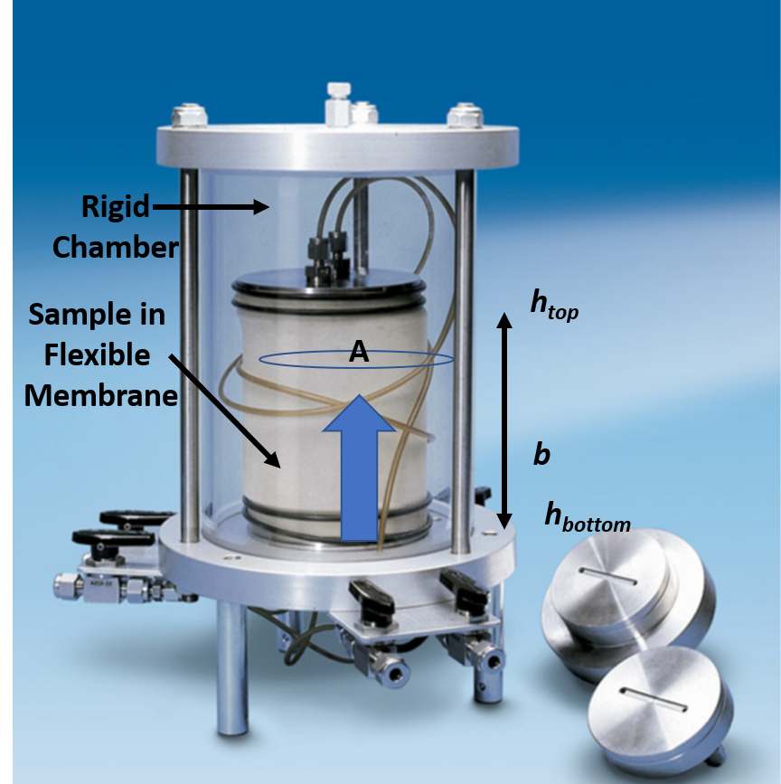
Figure Box 9‑2 ‑ Triaxial permeability cell. Valves and tubes shown connect to a control panel that supplies water, pressurization, vacuum, as well as methods to control gradients and measure flow rates. Water in the sample moves from the bottom to the top of the cell. A is the sample cross sectional area. The pressurized water in the rigid triaxial cell remains constant after being set by the user. The gradient is computed by subtracting the head at the top of the cell (htop, lower) from the head at the bottom of the cell (hbottom, higher), and dividing by the sample thickness, b. Kv is calculated after the flow rate reaches steady state (photograph modified from https://www.geo-con.com.au/product/permeability-cells/↗).
| [latex]K_{v} = \frac{Q}{i\ A}[/latex] | (Box 9‑2) |
|---|
where:
| Kv | = | hydraulic conductivity (LT‑1) |
|---|---|---|
| Q | = | constant discharge rate (L3T‑1) |
| i | = | hydraulic gradient, (head at the outlet – head at the inlet) / sample thickness, b, (negative value) (dimensionless) |
| A | = | cross sectional area of the sample (L2) |
Box 9.3 Consolidometer
When designing and constructing foundations for buildings, one must account for settlement from lateral deformation of the soil and a gradual settling resulting from a volume change if pore water drains from the soil. In the case of saturated clay deposits, one‑dimensional compression is of concern. Consolidation considerations generally assume the particles themselves are incompressible such that changes in the volume of material are due to rearrangement of the particles in response to loading and drainage of fluid. It is generally assumed that drainage follows Darcy’s Law.
The consolidometer (or oedometer) test is used to generate relationships between consolidation pressures, changes in the void ratio of the soil, and variations in the soil’s coefficient of consolidation. Estimates of vertical hydraulic conductivity can also be derived for each loading increment as reported by Haneberg and others (1998). Components of the equipment are shown in Figure Box 9‑3.
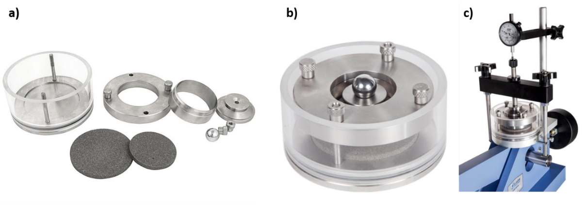
Figure Box 9‑3 ‑ Consolidometer set up and components. a) The chamber is fitted with a porous stone, filter paper, the saturated sample, filter paper and a second porous stone, and then secured with an outer ring. b) The chamber with the top compression piston installed. c) The chamber placed in an apparatus that applies varied consolidation pressures (black bar) using a lever and weights (not shown). The gauge measures the change in sample thickness. A saturated sample is allowed to drain and water discharge can be measured. (photographs from: a) https://certifiedmtp.com/karol-warner-1240-d-2-42in-fixed-ring-consolidometer/↗; b) https://www.globalgilson.com/100mm-fixed-ring-consolidometer↗; c) https://www.globalgilson.com/lever-loaded-consolidation-frame↗).
The coefficient of consolidation, Cv, is determined from testing and relates to the rate of consolidation in response to a change in pressure. It is derived from interpretation of sample condition changes and is often interpreted from graphical plots of where the time associated with changes in 50 percent or 90 percent of the sample thickness are identified (Wray, 1986). The saturated hydraulic conductivity can be computed for each load increment (Terzaghi, 1943; Das, 1983) as shown in Equations Box 9‑3 and Box 9‑4.
| [latex]K_{v} = \frac{a_{v}\gamma}{1 - e}[/latex] | (Box 9‑3) | |
|---|---|---|
| [latex]a_{v} = \frac{e_{1} - e_{2}}{\left( p_{2} - p_{1} \right)}[/latex] | (Box 9‑4) |
where:
| Kv | = | permeability at a specified time (LT‑1) |
|---|---|---|
| Cv | = | coefficient of consolidation (L2T‑1) |
| av | = | change in void ratio divided by the change in pressure at specified time increment (LT2M‑1) |
| e1 | = | void ratio at pressure p1 (dimensionless) |
| e2 | = | void ratio at pressure p2 (dimensionless) |
| p1 | = | compression pressure applied to the sample (M(L‑2T‑1) |
| p2 | = | compression pressure applied to the sample (ML‑2T‑1) |
| γ | = | specific weight of water (ML‑2T‑2) |
Petersen (1956) modified the consolidation testing apparatus to directly measure hydraulic conductivity at different pressure increments using a falling head permeameter. He found a good correlation with computed values of Kv and falling head derived values.
Olsen and others (1991) published innovations in measuring hydraulic conductivity using a one‑dimensional consolidometers and triaxial cells. In both cases a flow pump creates a constant flow from the sample base that is established from a pressure‑controlled reservoir (Figure Box 9‑4). Pressure differences are measured, a gradient computed, and Kv is calculated using Darcy’s Law (Equation Box 9‑2).
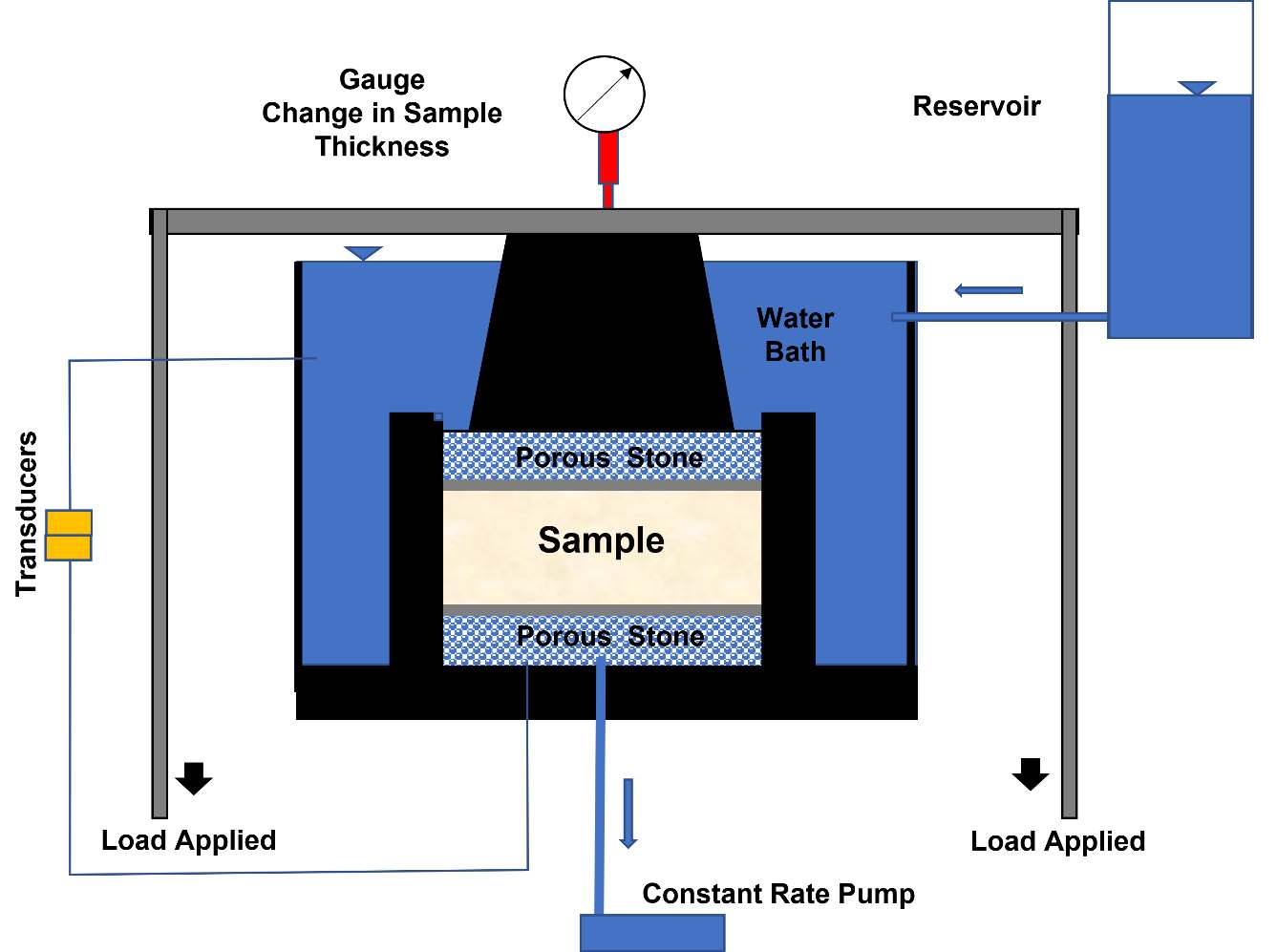
Figure Box 9‑4 ‑ Consolidometer set up with a constant rate pump. Gauge measures the change in sample thickness. Transducers measure the head at the base and top of the sample and the constant rate pump controls the flow rate through the sample. The reservoir provides a constant head to the water bath that is in communication with the sample.