
12.3 Steady‑State Approximation of Transmissivity
Pumping a well until steady‑state conditions are generated allows for application of steady‑state equations to solve for T. The pumping rate, the radius of the pumping well, and an estimate of the radial distance where drawdown is zero are needed to estimate T. The steady‑state drawdown in the pumping well needs to be corrected for partial penetration and well losses so that it more closely represents formational drawdown. If this is not done T and K estimates will be underestimated as the observed drawdown at the well is lower than if only formational properties were controlling the pumping water level as shown in Figure 93.
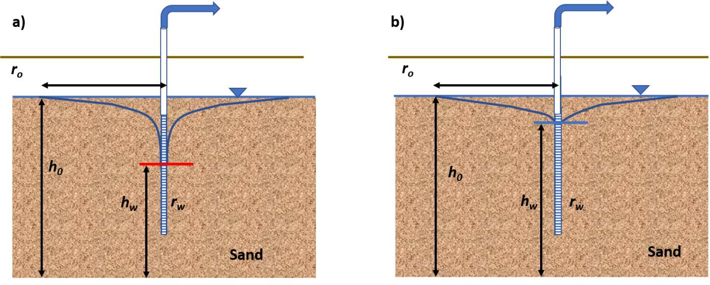
Figure 93 ‑ Unconfined sand aquifer with a single pumping well. The saturated thickness of the aquifer at the well of radius rw is hw and the saturated thickness at the radial distance r0 where drawdown is zero is h0. Values of h are measured from the aquifer base. a) The pumping level is impacted by well loss and partial penetration. b) Pumping‑well drawdown is corrected for the effects of partial penetration and well loss.
The Thiem equation describing the relationship of the steady‑state drawdown at two radial distances for unconfined and confined conditions is presented in Equation (97) and Equation (98), respectively, with Figure 94 presenting the parameters for confined aquifer systems. The corrected drawdown is paired with the well radius. For unconfined conditions, an arbitrary radial distance of 250 m is often used for the zero‑drawdown distance and for confined aquifers an arbitrary value of 500 m is used.
| [latex]K = \frac{Q}{\pi\left( h_{0}^{2} - h_{w}^{2} \right)}\ln\left( \frac{r_{0}}{r_{w}} \right)[/latex] | (97) |
|---|
where:
| [latex]T = \frac{Q}{2\pi\left( h_{0} - h_{w} \right)}\ln\left( \frac{r_{0}}{r_{w}} \right)[/latex] | (98) |
where:
| T | = | confined aquifer transmissivity (Kb) (L2T‑1) |
|---|---|---|
| Q | = | constant pumping rate (L3T‑1) |
| h0 | = | head at the radial distance where drawdown is zero (L) |
| hw | = | head at the pumping well (L) |
| r0 | = | radial distance at which drawdown is zero (L) |
| rw | = | radius of the pumping well (L) |
The well radius is represented by the effective radius (screen radius + gravel pack radius) when a gravel pack is present.
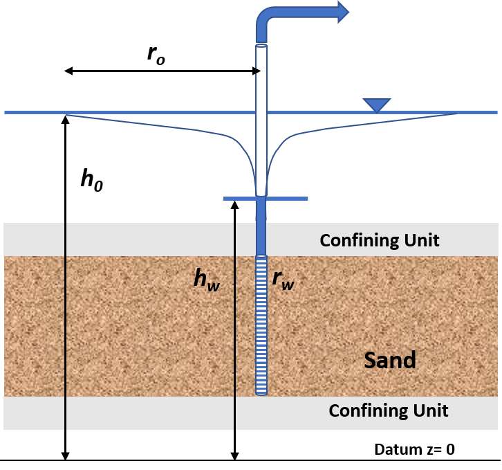
Figure 94 ‑ Defining parameters for a steady‑state single well pumping test in a confined aquifer. The head value, hw, is assigned to the radius of the pumping well, rw, and the head value, h0, assigned to the radial distance, r0, where no drawdown occurs, are measured from a horizontal datum. The pumping well drawdown requires correction for partial penetration and well loss.
Example
A single well penetrating a confined aquifer is pumped for 8 hours at a rate of 1000 m3/d. The head at the pumping well with a radius of 0.05 m seems to have stabilized at 856.8 m. The static head at the beginning of the test is 879.1 m. Analysis of the partial penetration and well loss effects suggest they contribute an additional 8.4 m to the measured head. Compute T for the aquifer.
The head at rw equals 856.8 m + 8.4 m = 865.2 m. The value is added because the measured head value (not drawdown) is lower than if only formational properties affected the response. At an estimated radial distance of 500 m (r0) the head is equal to the static water level, 879.1 m. Then T is calculated using Equation (98).
[latex]T = \frac{1000\frac{m^{3}}{d}}{2\ (3.14)\ (879.1\ m - 865.2\ m)}\ln\left( \frac{500\ m}{0.05\ m} \right) = 105.5\ \frac{m^{2}}{d}[/latex]