
Solution Exercise 2
A pumping test is conducted on a production well located in an extensive, isotropic, and homogeneous, 25‑m thick, totally confined, sand and gravel aquifer. The production well has a 15 m screened interval. The well was pumped at a constant rate of 1,200 m3/d for 240 minutes. Time‑drawdown data were collected at three observation wells located 61 m, 122 m, and 244 m from the pumping well as shown in the image below. An Excel® data base of the time‑drawdown data is available on the web page for this book↗.
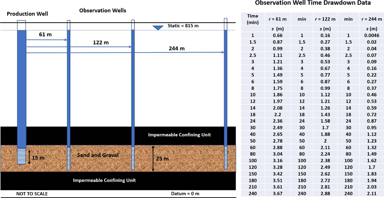
Information related to Exercise 2. A production well is pumped at a constant rate in a totally confined isotropic and homogeneous aquifer that is infinite in lateral extent. Time‑drawdown data are collected from three observation wells. Configuration of the pumping well location, screen length and location of the observation wells are shown in cross section. Time‑drawdown data sets for the three observation wells are presented (modified from Lohman, 1972).
- Prepare log‑log pots of the time‑drawdown data for each of the observation wells. Using manual or automated curve matching, determine values of transmissivity and storativity for each data set.
The Theis equation and curve matching was applied to determine T and S using Equations (28) and (29) from Section 8.1.
[latex]T = \frac{Q}{4\pi s}\ W(u)[/latex]
[latex]S = \frac{u4Tt}{r^{2}}[/latex]
Manual curve matching was applied. Observation well data sets were plotted as log‑log plots in Excel®. The Excel® plot was copied into a slide in Microsoft PowerPoint®. The type curve for totally confined conditions, W(u) versus 1/u (Figure 28 of Section 8) was copied and imported into PowerPoint. The Excel® time‑drawdown data plot was made transparent by right clicking on the chart (log‑log data plot) and then going to (Format chart area). The transparency was then maximized. Next the x and y axes were stretched and adjusted to have the Excel® plot axes match the type curve axes (same area represented by each change in major axis (1 to 10, 10 to 100, etc.). Once the data plot was adjusted to the same scale as the type curve it was maneuvered to find the best fit of the data to the type curve while keeping the axes parallel. Next a match point in the overlapping plot area was selected and values of s, t, W(u) and 1/u were determined.
An image resulting from the curve matching process is shown here for the observation well at r = 61 m with Q = 1,200 m3/d.
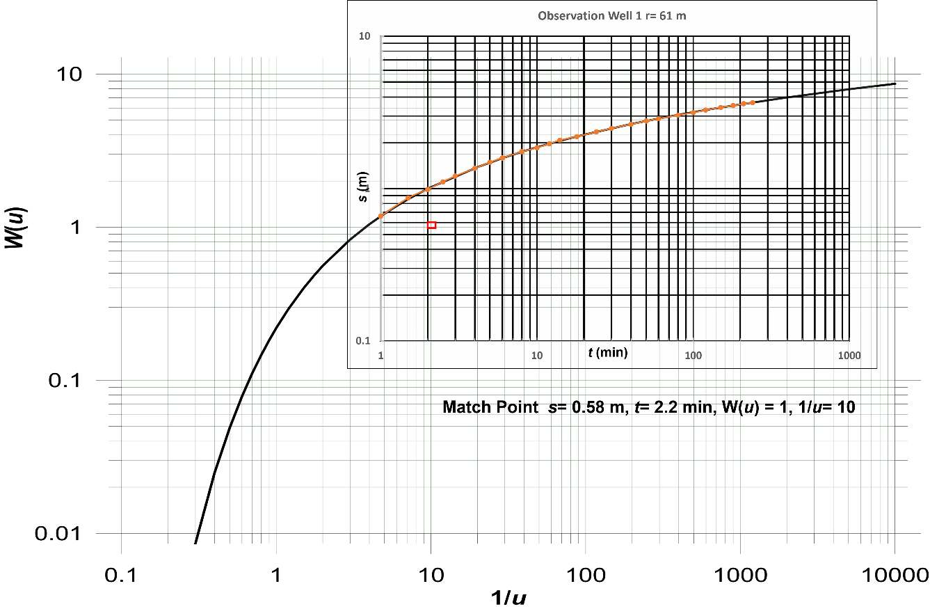
Curve matching for the observation well located at r = 61 m. The dark black line is the Theis type curve (W(u) and 1/u axes). The orange dots and line represent the field data. The red square is the location of the match point.
Match point: s = 0.58 m, t = 2.2 min, W(u) = 1 and 1/u = 10 (u = 0.1)
[latex]T = \frac{Q}{4\pi s}\ W(u) = \frac{1200\ \frac{m^{3}}{d}}{4\ (3.14)\ 0.58\ m}\ (1)\ = \ 165\ \frac{m^{2}}{d}[/latex]
[latex]S = \frac{u4Tt}{r^{2}} = \frac{0.1\ (4)\ 165\ \frac{m^{2}}{d}2.2min\frac{1\ d}{1440\ min}}{{(61\ m)}^{2}}\ = 0.00003\ \ or\ 3x10^{- 5}[/latex]
An image resulting from the curve matching process is shown here for the observation well at r = 122 m with Q = 1,200 m3/d.
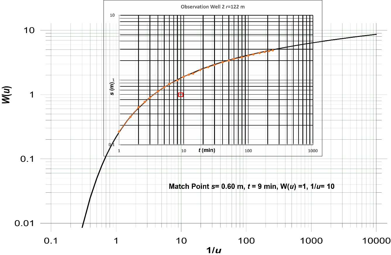
Curve matching for the observation well located at r = 122 m. The dark black line is the Theis type curve (W(u) and 1/u axes) and the orange line represents the field data. The red square is the location of the match point.
Match point: s = 0.6 m, t = 9.0 min, W(u) = 1 and 1/u = 10 (u = 0.1)
[latex]T = \frac{Q}{4\pi s}\ W(u) = \frac{1200\ \frac{m^{3}}{d}}{4\ (3.14)\ 0.6\ m}\ (1)\ = \ 159\ \frac{m^{2}}{d}[/latex]
[latex]S = \frac{u4Tt}{r^{2}} = \frac{0.1\ (4)\ 159\ \frac{m^{2}}{d}9\ min\frac{1\ d}{1440\ min}}{{(122\ m)}^{2}}\ = 0.00003\ \ or\ 3x10^{- 5}[/latex]
An image resulting from the curve matching process is shown here for the observation well at r= 244 m, Q = 1,200 m3/d.
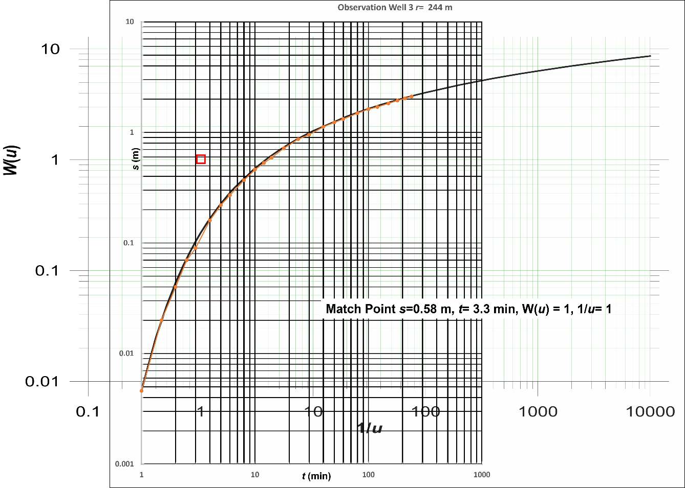
Curve matching for the observation well located at r = 244 m. The dark black line is the Theis type curve (W(u) and 1/u axes) and the orange line represents the field data. The red square is the location of the match point.
Match point: s = 0.58 m, t = 3.3 min, W(u) = 1 and 1/u = 1 (u = 1)
[latex]T = \frac{Q}{4\pi s}\ W(u) = \frac{1200\ \frac{m^{3}}{d}}{4\ (3.14)\ 0.58\ m}\ (1)\ = \ 165\ \frac{m^{2}}{d}[/latex]
[latex]S = \frac{u4Tt}{r^{2}} = \frac{1\ (4)\ 165\ \frac{m^{2}}{d}3.3\ min\frac{1\ d}{1440\ min}}{{(244\ m)}^{2}}\ = 0.00002\ \ or\ 2x10^{- 5}[/latex]
- Compare and contrast the values computed. Should they all be the same? If not, how would you present the results to the well owner?
Given that the observation wells are more than two aquifer thicknesses from the pumping well there should not be any partial penetration effects, so if the aquifer is truly isotropic and homogeneous then the values should all be the same. For this example, they are all very close. Differences in computed values may have originated from errors in field measurements of s, t, and Q, when constructing and matching the curves, and when selecting the match points.
The best way to present the results to the well owner would be to average and round the T and the S values, Tavg = 163 m2/d rounded to 160 m2/d; Savg = 0.000027 rounded to 0.00003.
- Analysis of pumping a confined aquifer can also be accomplished using the Cooper‑Jacob straight line method. The process is to plot the time‑drawdown data for the observation well located 122 m from the pumping well as a semi‑log plot and determine T and S. Compare these results to the results from the part (a) type curve analyses, and comment on their similarity or differences.
The data set for the observation well located at r = 122 m is plotted as a semi‑log graph in the image shown here.
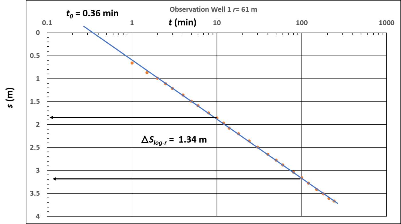
Semi log plot of time‑drawdown data for r = 122 m. ∆slog-t was determined over one log cycle of time (10 to 100 minutes) and t0 is derived from where the fitted line crosses the zero‑drawdown line.
[latex]T = 2.3\frac{Q}{4\pi\Delta s} = 2.3\frac{1200\ \frac{m^{3}}{d}}{4\ (3.14)\ 1.34\ m} = 164\frac{m^{2}}{d}[/latex]
[latex]S = 2.25\frac{Tt_{0}}{r^{2}} = 2.25\frac{164\frac{m^{2}}{d}\ 0.36\ min\frac{1\ d}{1440\ min}}{{(122\ m)}^{2}} = 0.000006\ or\ 6x10^{- 6}[/latex]
The T value is very similar to the values computed from curve matching. The storativity is lower than the values derived from the curve match. Both values can be represented by 0.00001.
- The confined time‑drawdown data can also be interpreted using the distance‑drawdown method. Make a semi‑log plot of the distance‑drawdown data at 100 minutes and calculate T and S. Compare these results to those derived from type curve and time‑drawdown straight line analyses. Discuss why the values are similar or different.
A semi‑log distance‑drawdown plot at 100 min is presented in the image here.
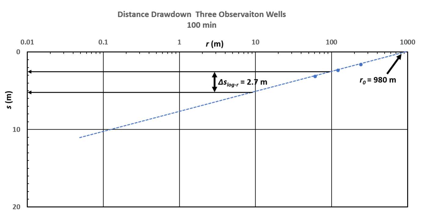
A semi‑log distance‑drawdown plot of the observation well data at 100 minutes. ∆slog-r is computed over one log cycle of distance. A dashed trend line is added. r0 is the radial distance where drawdown is zero.
The Cooper‑Jacob equations used to analyze the distance‑drawdown data are Equations (37) and (38) from Section 8.3.3.
[latex]T = \frac{2.3\ Q\ }{2\ \pi\ {\Delta s}_{log - r}} = \frac{2.3\ \left( 1200\ \frac{m^{3}}{d} \right)\ }{2\ (3.14)\ 2.7\ m} = 163\frac{m^{2}}{d}[/latex]
[latex]S = 2.25\ \frac{Tt}{r_{0}^{2}} = 2.25\ \frac{163\frac{m^{2}}{d}\ 100\ min\frac{1\ d}{1440\ min}}{{(980\ m)}^{2}} = 0.00003\ \ or\ \ 3x10^{- 5}[/latex]
These values are very similar to those obtained from curve matching and the application of the time‑drawdown semi‑log plot. The storativity value interpreted from the semi‑log, distance‑drawdown plot was similar to curve matching results. All in all, the manual plotting and interpretations were very similar.
- Using the distance‑drawdown plot examine the efficiency of the production well. If the production well diameter is 0.20 m and the drawdown at 100 minutes in the pumping well is 12.34 m, what is the efficiency of the pumping well (i.e., measured drawdown divided by theoretical drawdown)?
The straight trend line on the distance‑drawdown plot can be extended to include the radius of the pumping well (0.1 m) as shown below.
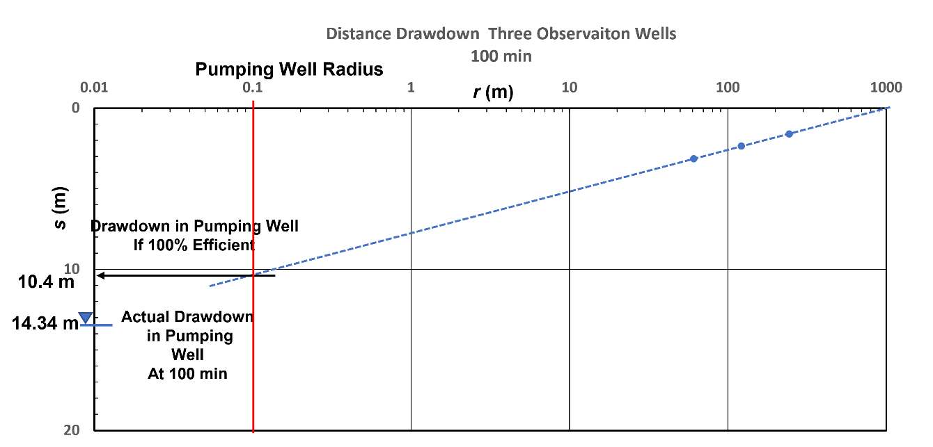
Semi‑log distance‑drawdown plot at 100 minutes used to assess pumping well efficiency. The red line shows the pumping well radius. The corresponding theoretical drawdown (sF) is 10.4 m.
The efficiency, E, of a pumping well is defined as the theoretical drawdown (sF) at a fixed time divided by the observed drawdown or total drawdown, sF/sT. In this setting the well efficiency equals 10.4 m / 14.34 m = 0.72 or 72 percent. The well efficiency represents conditions when the well is pumping at 1,200 m3/d. In an inefficient well the amount of well loss that occurs (additional drawdown resulting from the hardware design and pumping rate) increases with the pumping rate. So, if the well yield is increased by 50 percent, a separate analysis would be required to determine the well efficiency at the higher pumping rate.
- The well is planned to be used to supplement the city water system. After a seasonal supply evaluation, it was decided to pump the well for 200 days at a constant rate of 1,000 m3/d. There are other wells in the area and a regulatory agency wants to know if other wells would be affected when this well is pumped. Ignoring the effects of pumping in the other wells, what is the predicted drawdown 1000 m from the well at the end of the pumping period?
This new discharge rate and pumping schedule can be input into the Theis Equation (Equation (26)) to solve for the drawdown at 1,000 m from the pumping well. Based on the five testing results, using the mean, the transmissivity is set at 163 m2/d and the storativity at 2.3 x 10‑5. First, u, is calculated, then W(u) is read from Figure 26 and drawdown is calculated using Equation (26).
[latex]u = \frac{r^{2}S}{4Tt} = \frac{{(1000\ m)}^{2}\ \ 0.000023}{4\left( 163\frac{m^{2}}{d} \right)200\ d} = 0.0002[/latex]
Then using Figure 26 to look up, or WolframAlpha to solve W(u)=‑Ei(‑u), W(u) is 7.9402.
[latex]s(r,t) = \frac{Q}{4\pi T}\ W(u) = \frac{1200\ \frac{m^{3}}{d}}{4\ (3.14)\ 163\frac{m^{2}}{d}}\ 7.9402 = 4.65\ m[/latex]