
9.3 Hantush Equation for a Leaky Confined System with Water Released from Confining Bed Storage
When pumping a confined aquifer with a permeable confining bed contributing water to the pumped aquifer, the reduction in head in the aquifer creates a hydraulic gradient in the confining bed toward the aquifer. As heads in the confining bed are lowered, water is released from storage and flows to the confined aquifer. If the confining bed is relativity thin, the gradient change reaches the top of the bed relatively quickly and then stabilizes such that release of water from storage within the confining bed ceases. If there is an aquifer on the other side of the confining bed, it provides a source of water that flows through the confining bed to the pumped aquifer. Hantush (1960) developed a set of analytical solutions that account for leakage of water from aquitard storage into a confined aquifer as it is pumped. His work also addresses leakage into a confined system from vertical flow though confining beds as described by Hantush‑Jacob and illustrated in Figure 41. Conceptual models of such leakage are illustrated in Figure 49.
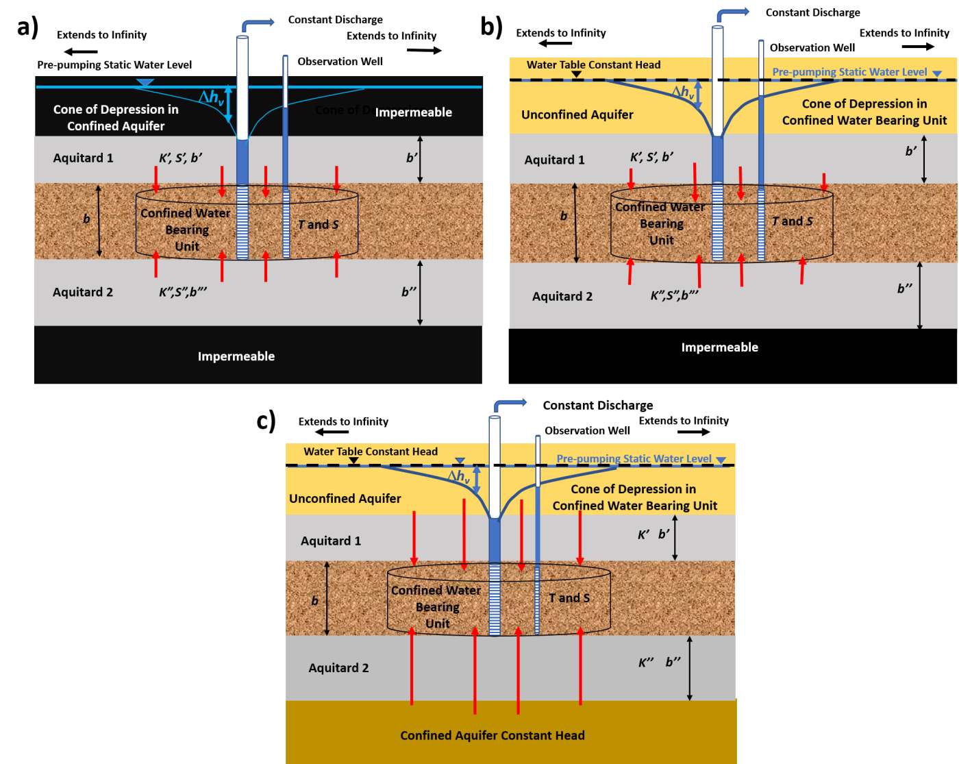
Figure 49 ‑ Conceptual models that can be represented by the Hantush equation (1960).
a) Drawdown in a confined aquifer that receives water from storage in one or two confining beds when the beds overlying and underlying the confining beds are not permeable.
b) Drawdown in a confined aquifer that receives water from storage in overlying and/or underlying confining beds, as well as leakage of water through the confining bed from a highly transmissive unit such as an unconfined water table aquifer.
c) Drawdown in a confined aquifer receiving water via direct flow through a confining bed that has negligible storage from a highly transmissive aquifer above and/or below the confining bed.
The general analytical solution for leaky conditions given by Hantush (1960) is presented in Equation (55). The different conditions shown in Figure 49 can be represented using variations of this equation. Similar to the Theis well function for drawdown when pumping a fully confined water bearing unit, the Hantush integral includes an infinite series and can be represented using an approximation as shown in Equation (56). The Hantush well function uses the parameter b to account for the relative properties of the aquifer and its overlying and underlying layers. Drawdown in a confined unit with one or two adjacent confining unit(s) that release(s) water from storage that is overlain or underlain by an impermeable unit is calculated as shown in Equation (57).
| [latex]s(r,t) = \frac{Q}{4\pi T}\ \int_{u}^{\infty}{\ \frac{1}{y}\ exp\ \left\{ - y \right\}\ erfc\left( \frac{\frac{\beta}{\sqrt{u}}}{\sqrt{y(y - u}\ )} \right)}dy[/latex] | (55) | |
|---|---|---|
| [latex]H(u,\beta) = W(u) - \ \frac{4\beta}{(\pi{u)}^{0.5}}\ \left\lbrack 0.2577 + 0.6631\exp\left( \frac{- u}{2}\ \right) \right\rbrack[/latex] | (56) | |
| [latex]s(r,t) = \frac{Q}{4\pi T}\ H(u,\beta)[/latex] | (57) |
where:
| s(r,t) | = | drawdown at a radial distance r and time t (L) |
|---|---|---|
| r | = | radial distance to the observation well (L) |
| t | = | time (T) |
| Q | = | constant well discharge rate (L3T‑1) |
| T | = | transmissivity of the confined pumped unit (L2T‑1) |
| y | = | variable of integration |
| erfc | = | complementary error function (dimensionless) |
| β | = | represents the relative transmissibly and storage of the pumped unit and the contributing overlying and/or underlying units as shown in Equations (58) and (59) (dimensionless) |
| u | = | r2S/(4Tt) |
| H(u,β) | = | Hantush well function integral (dimensionless) |
| W(u) | = | Theis well function (dimensionless) |
When storage comes from only one confining bed, b is described by Equation (58). This represents the case illustrated in Figure 49a with one aquitard—which can be above or below the pumped unit. In this case the other aquitard shown in Figure 49a is impermeable. For the setting with two confining beds, b includes terms for both aquitards and is described by Equation (59).
| [latex]\beta = \frac{r}{4\ }\sqrt{\frac{K'S'}{b'TS}\ }[/latex] | (58) |
|---|
| [latex]\beta = \frac{r}{4\ }\left( \sqrt{\frac{K'S'}{b'TS}\ }\ + \sqrt{\frac{K"S"}{b^{"}TS}} \right)[/latex] | (59) |
|---|
where:
| r | = | radial distance to the pumping well (L) |
|---|---|---|
| K’ | = | vertical hydraulic conductivity of the first confining unit (LT‑1) |
| K” | = | vertical hydraulic conductivity of the second confining unit (LT‑1) |
| S’ | = | storativity of the first confining unit (dimensionless) |
| S” | = | storativity of the second confining unit (dimensionless) |
| b’ | = | thickness of the first confining unit (L) |
| b” | = | thickness of the second confining unit (L) |
| T | = | transmissivity of the confined unit being pumped (L2T‑1) |
| S | = | storativity of the confined unit being pumped (dimensionless) |
Drawdown in the confined aquifer can be calculated with Equation (57) by using Equation (56) to calculate the Hantush well function (H(u,β)) or reading/interpolating the value from a table (Figure 50) or type curves (Figure 51).
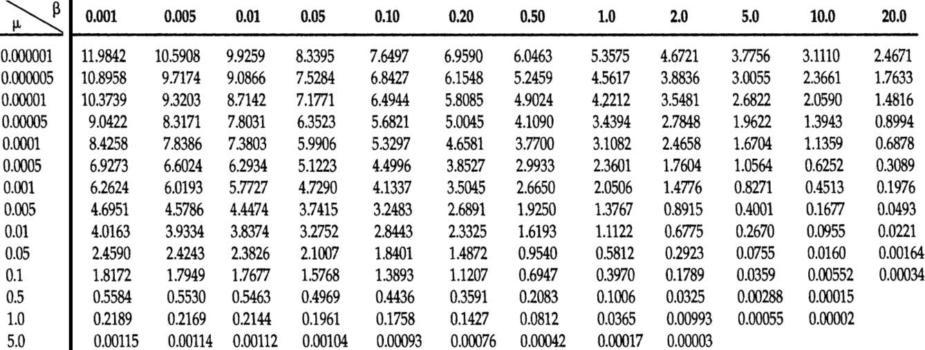
Figure 50 ‑ Tables of the Hantush well function for variables u and β (from Fetter (2001)). Type curves of H(u,β) versus 1/u are illustrated in Figure 51.
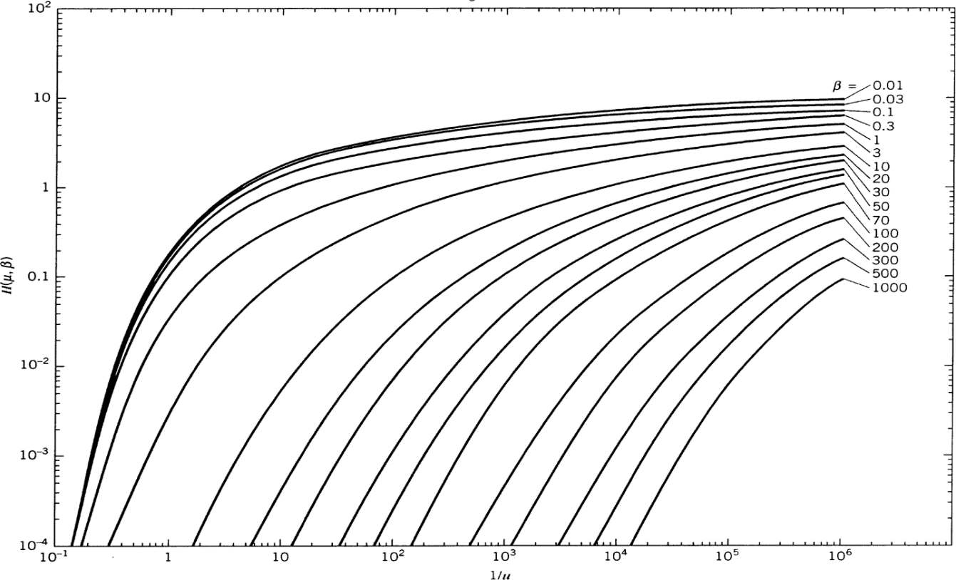
Figure 51 ‑ Type curves of H(u,β) versus 1/u plotted on log‑log axes (modified from Reed (1980); Kruseman & de RIdder (2000); Kasenow (2001)).
The table of values (Figure 50) and plotted type curves (Figure 51) represent a subset of H(u,β) values that can be generated by substituting combinations of u and β into Equation (56) or by using mathematical software packages to solve the integral portion of Equation (55). The required values are commonly interpolated from the table or curves presented in Figure 50 and Figure 51 respectively.
Using the Hantush Equation to Predict Drawdown in Leaky Confined Units with Water Released from Confining Bed Storage
When the hydraulic properties of the sequence of geologic units as illustrated in Figure 49a are known, the Hantush equation can be used to approximate drawdown at an observation point at any time t after the pumping commenced.
Example
A fully penetrating well pumps at 500 m3/d for 0.2 d from a 30 m thick leaky confined sand rich aquifer that is overlain by a silt rich aquitard that is 20 m thick. The confining units are overlain and underlain by impermeable units (Figure 49a). The observation well is located 53 m from the pumping well. The transmissivity of the confined aquifer is 300 m2/d and the storativity is 0.00003. The vertical hydraulic conductivity of the confining bed is 0.3 m/d and the storativity of the confining bed is 0.00001. Calculate the drawdown in the observation well after 0.2 d of pumping.
Using the definition of u (u=r2S/(4Tt)) along with Equations (58) and (60), and the information listed above, H(u,b) is obtained by first computing u and , and then using Figure 50 to obtain the Hantush well function.
[latex]u = \frac{r^{2}S}{4Tt} = \frac{{(53\ m)}^{2}\ 0.00003}{4\ \left( 300\frac{m^{2}}{d} \right)0.2\ d} = 0.0004[/latex]
[latex]\beta = \frac{r}{4\ }\sqrt{\frac{K'S'}{b'TS}\ } = \frac{53\ m}{4\ }\sqrt{\frac{0.3\frac{m}{d}(0.00001)}{20\ m\ \left( 300\frac{m^{2}}{d} \right)\ 0.00003}} = 0.05[/latex]
With u = 0.0004 and b = 0.05, H(u,b) is obtained by interpolation from Figure 50 or Figure 51. With u = 0.0004, b = 0.05 then H(u,b) is about 6.52.
| u | β | H(u,β) |
|---|---|---|
| 0.0001 | 0.05 | 7.1771 |
| 0.0004 | 0.05 | 6.52 (interpolated) |
| 0.0005 | 0.05 | 6.3523 |
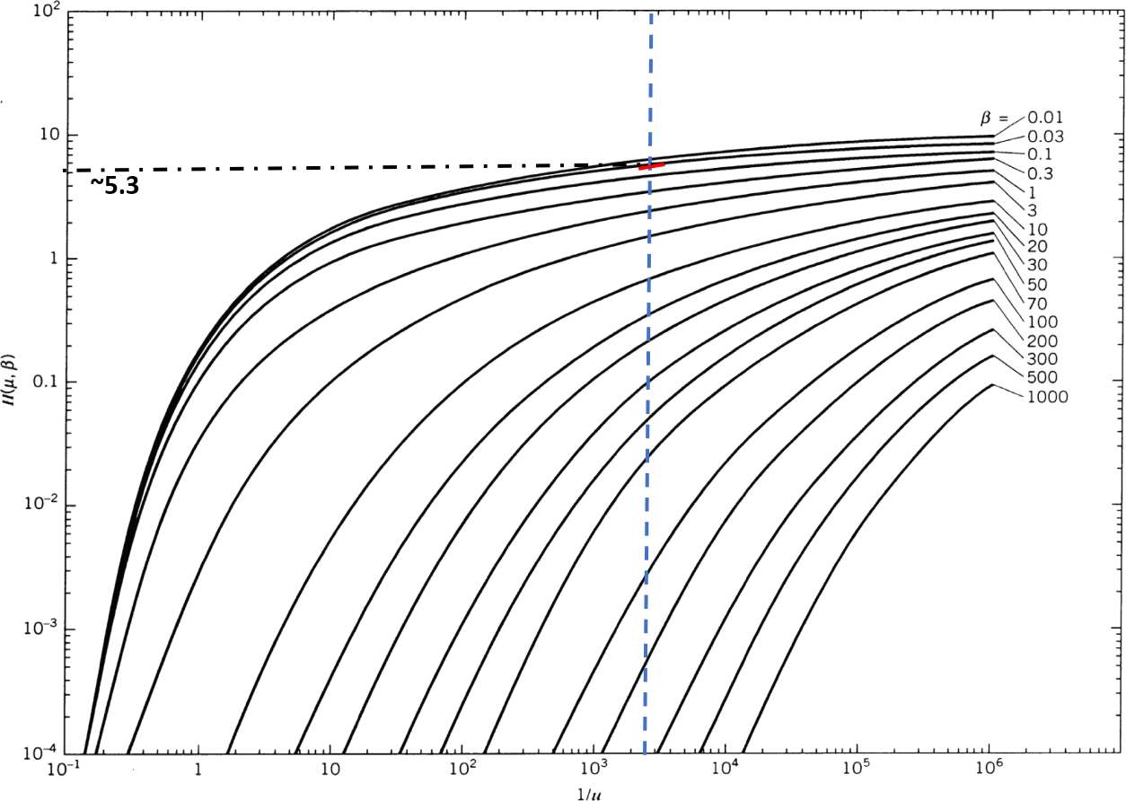
Figure 52 ‑ Hantush type curves plotted on log‑log scales. The dashed vertical blue line is the computed value of 1/u (2,500) for the example problem. The red line is the interpolated value of β, about 0.05, and the black dot dashed line is the interpolated value of H(u,β), about 5.3. This value is lower than derived from the tables. The close plotting of the type curves made interpretation difficult for the designated β value (modified from Kruseman & de RIdder, 2000; Kasenow, 2001).
Then Equation (57) provides the value of drawdown.
[latex]s(r,t) = \frac{500\frac{m^{3}}{d}}{4\ (3.14)\ 300\frac{m^{2}}{d}}\ 6.52 = 0.87\ m[/latex]
Hantush Curve Matching Method to Compute T and S from a Pumping Test in Leaky Confined Unit with Aquitard Storage
The Hantush equation can be used to determine T and S from time‑drawdown data collected in an observation well when a leaky confined aquifer is pumped and water is released from aquitard storage. The hydraulic conductivity and storage properties of adjacent confining units can also be derived. Standard curve‑matching techniques described in Section 8.3.1 can be used.
After data from a pumping test has been collected, T and S for a leaky confined aquifer with the release of water from confining bed storage is estimated by first plotting drawdown versus time on a log‑log graph at the same scale as the type curves as shown in (Figure 53).
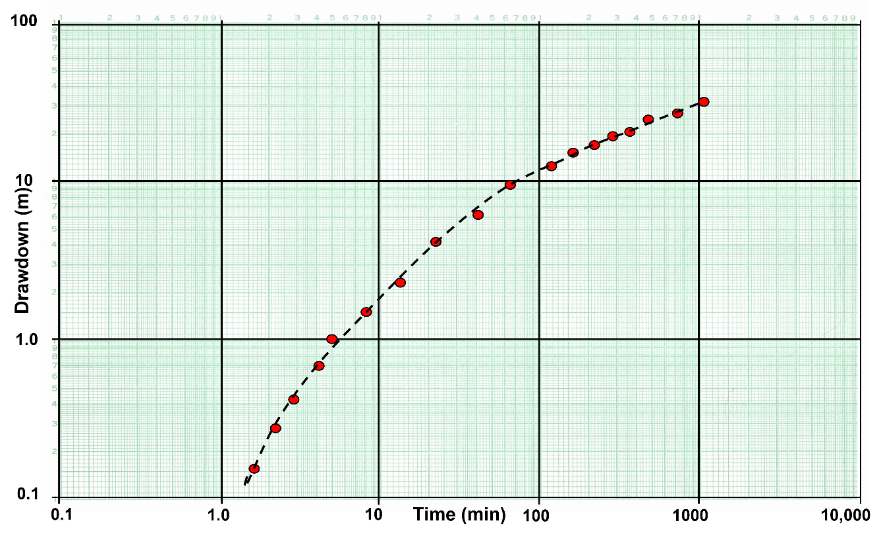
Figure 53 ‑ Log‑log plot of the response of an observation well to the pumping of a well in a leaky confined aquifer with water being released from confining bed storage.
The data graph (Figure 53) is overlain on the type curves (Figure 51). Keeping the axes parallel, the field data graph and type curve graph are overlain and shifted until the curves match (Figure 54). A match point is selected from the overlapping portion of the two plots and values of H(u,β), 1/u, s, t and β are obtained. Estimates of T and S for the leaky confined unit as well as its hydraulic conductivity, and, at early times, storativity values of the confining beds can be estimated using Equations (60) and (61) which are obtained from rearranging Equation (57) and the definition of u (u=r2S/(4Tt)), respectively. Early time refers to the period after pumping begins when the confining unit is releasing water from storage. Early time is less than b’S’/10K’.
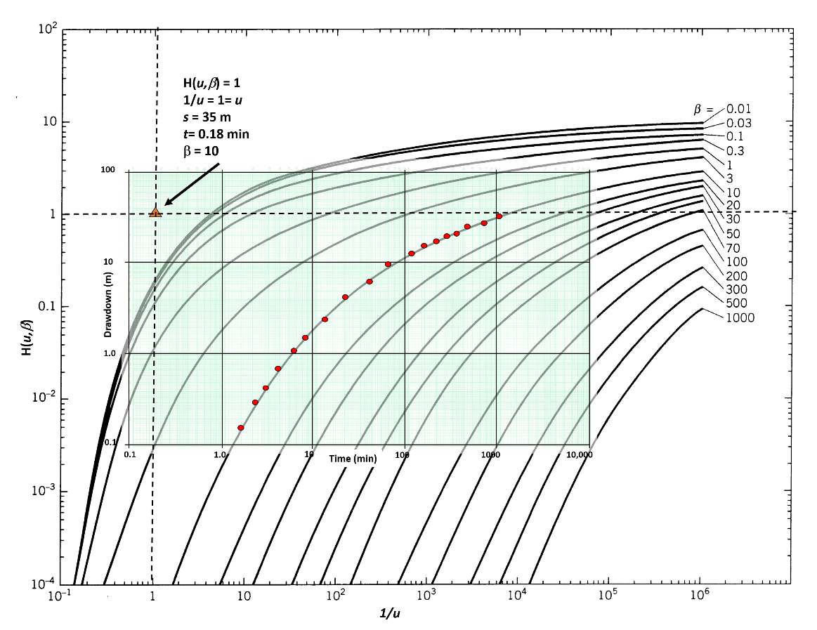
Figure 54 ‑ Curve matching of the data from an observation well with the Hantush type curves. The scales of both graphs are equal and their axes are kept parallel. The value of β is obtained from the corresponding curve and the match point values are obtained at the location of the orange triangle (modified from Reed, 1980; Kruseman & de Ridder, 2000).
| [latex]T = \frac{Q}{4\pi s}\ H(u,\beta)[/latex] | (60) | |
|---|---|---|
| [latex]S = \frac{u(4Tt)}{r^{2}}[/latex] | (61) |
where:
| T | = | transmissivity (L2T‑1) |
|---|---|---|
| s | = | drawdown (L) |
| Q | = | constant pumping rate (L3T‑1) |
| H(u,β) | = | Hantush Well Function (dimensionless) |
| u | = | r2S/(4Tt) (dimensionless) |
| r | = | radial distance to the observation well (L) |
| t | = | time since pumping started (T) |
| S | = | storativity of the confined aquifer (dimensionless) |
Once T and S are computed for the pumped confined aquifer, estimates of the vertical hydraulic conductivity and storage properties of the confining unit can be derived as described by Schwartz and Zhang (2003). For conditions shown in Figure 49a, when K”b”S” = 0 then K’S’ is calculated using Equation (62) which is a rearrangement of Equation (58). When K”S”=K’S’ (Figure 49a) then K’S’ is calculated using Equation (63) which is a rearrangement of Equation (59) .
| [latex]K'S' = \ \frac{16\ b'TS\beta^{2}}{r^{2}}[/latex] | (62) | |
|---|---|---|
| [latex]K'S' = \ \frac{16\ TS\beta^{2}}{r^{2}}\ \left( \frac{b'b"}{\text{b' + b"} + 2(b'b")^{0.5}} \right)[/latex] | (63) |
where:
| β | = | defined by Equation (58) for Equation (62), and Equation (59) for Equation (63) |
|---|---|---|
| r | = | radial distance to the pumping well (L) |
| S’ | = | storativity of the first confining unit (dimensionless) |
| S” | = | storativity of the second confining unit (dimensionless) |
| S | = | storativity of the confined unit being pumped (dimensionless) |
| T | = | transmissivity of the confined unit being pumped (L2T‑1) |
| K’ | = | vertical hydraulic conductivity of the first confining unit (LT‑1) |
| b’ | = | thickness of the first confining unit (L) |
| K” | = | vertical hydraulic conductivity of the second confining unit (LT‑1) |
| b” | = | thickness of the second confining unit (L) |
Example
The data presented in Figure 54 represent drawdown in a fully‑penetrating observation well responding to a fully‑penetrating well in a confined aquifer that is pumped continuously for 1 day at 1,000 m3/d. The production well and observation well are completed in a 20 m thick sandstone unit. The observation well is 100 m from the pumping well. The confining unit overlying the leaky confined unit is a sandy shale that is 10 m thick. Based on this information and the curve matching results, the T and S of the confined sandstone unit can be computed as follows using Equations (60) and (61).
[latex]T = \frac{1000\ \frac{m^{3}}{d}}{4\ (3.14)\ 35\ m}\ (1) = 2.3\frac{m^{2}}{d}[/latex]
[latex]S = \frac{1\ (4)\ 2.3\frac{m^{2}}{d}0.000125\ }{{(100\ m)}^{2}} = \ 0.0000001\ or\ 1x10^{- 7}[/latex]
A rearrangement of Equation (58) is used to solve for hydraulic conductivity of the confining bed using either a known or estimated value for storativity of the confining bed. Methods to estimate the confined storativity are provided in Box 2. When the confining unit is fractured rock, Lohman (1972) suggests confining unit storativity can be estimated by multiplying the thickness of the unit in meters by 0.0000003/m. In this example the confining bed storativity is estimated as 10 m times 0.0000003/m and equals 0.000003. β from the curve match is 10. Then Equation (62) is rearranged to solve for K’.
[latex]K' = \ \frac{16\ b'TS\beta^{2}}{S'r^{2}} = \ \frac{16\ (10\ m)\ 2.3\frac{m^{2}}{d}(0.0000001)\ ({10)}^{2}}{(0.000003)\ {(100\ m)}^{2}} = 0.12\frac{m}{d}[/latex]