
Solution Exercise 7
A monitoring well that is 5.08 cm in diameter was installed in an unconfined silt‑rich formation that is 5 m thick. The base of the well screen is located 2.5 m below the land surface and is 1 m long. The water table is 0.5 m below land surface. A slug out test was performed on this well as illustrated in the image below.
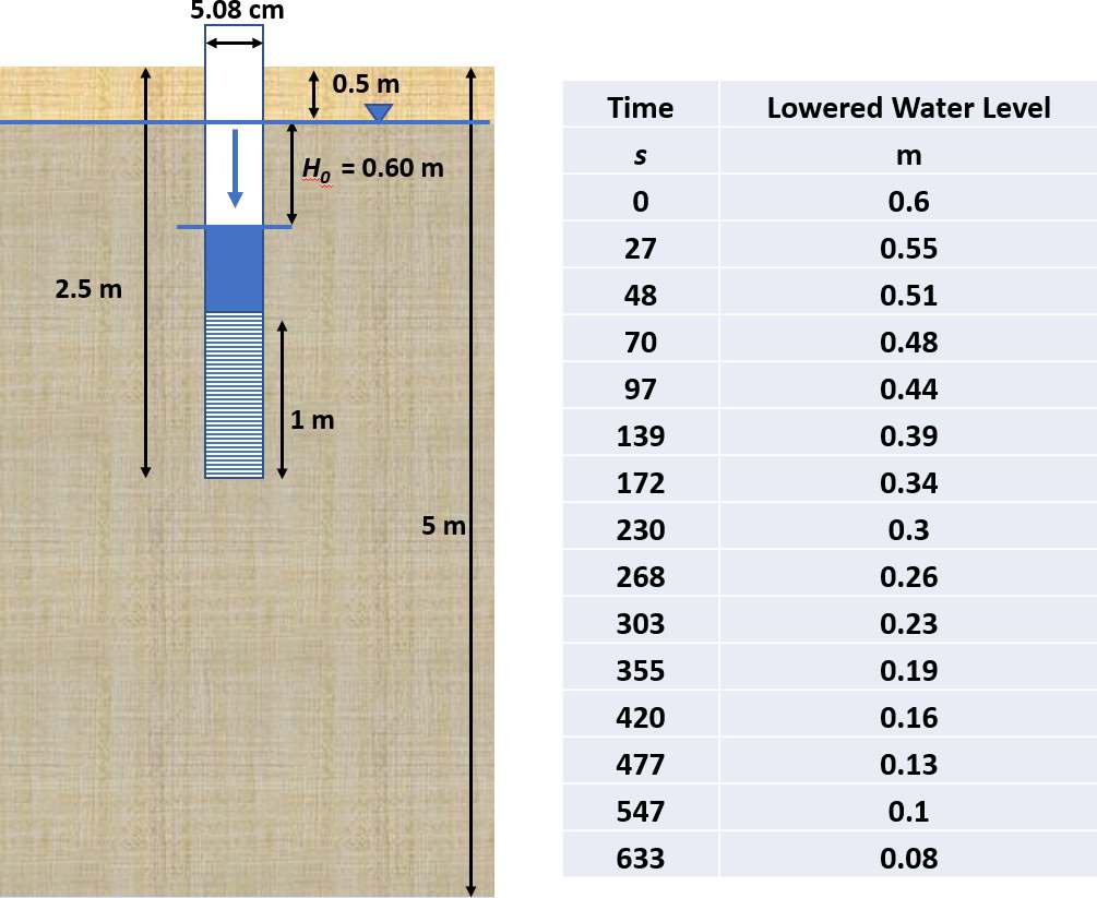
Slug out test conducted in a silt‑rich unconfined formation. a) Unpumped well design and location of screened interval. The slug test was conducted by lowering the water level by 0.6 m. This is the water level at the start of the test (H0). b) After 10.5 minutes (633 s) the water level had recovered within 0.08 m of the static water elevation (modified from Todd and Mays, 2005).
An Excel® data base of the time‑drawdown data is available on the web page for this book↗.
- Select an appropriate method to analyze the slug test data. Explain your choice.
- Use this method to calculate K.
As the slug test results are overdamped, either the Hvorslev method or Bouwer and Rice method would be applicable as discussed in Section 14. They both can be applied to unconfined conditions. The Hvorslev method is used for this solution.
The Hvorslev method can be defined using the slope of the unrecovered data plot or the T0.37 time as shown in Equations (107) and (108).
[latex]K = \frac{{r_{c}}^{2}\ln\left( \frac{L_{e}}{r_{s}} \right)}{2\ L_{e}\ \left( t_{2} - t_{1} \right)}\ln\left( \frac{h_{1}}{h_{2}} \right)[/latex]
[latex]K = \frac{{r_{c}}^{2}\ln\left( \frac{L_{e}}{r_{s}} \right)}{2\ L_{e}\ T_{.37}}[/latex]
A plot of the unrecovered head data is plotted against time as shown here.
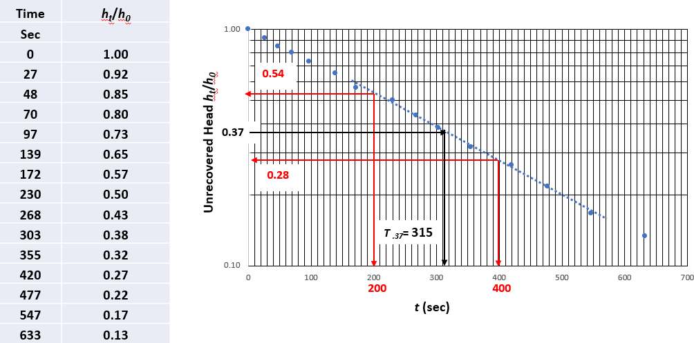
Slug test data and plot. a) Water level data converted to the ratio of unrecovered head (H0 = 0.6 m). b) Semi‑log plot of unrecovered head ratio versus time. The solid black line is fitted to the data.
Parameters for the Hvorslev equations are calculated and listed here.
[latex]r_{c} = r_{s} = \frac{5.08\ cm}{2} = 2.54\ cm[/latex]
Le is the length of the screen.
Le = 1 m
[latex]\frac{h_{1}}{h_{2}} = \frac{0.54\ m}{0.28\ m} = 1.9[/latex]
[latex]t_{2\ } - t_{1} = 400\ sec\ - 200\ sec = 200\ sec\ \frac{1\ d}{86400\ sec} = 0.0023\ d[/latex]
[latex]K = \frac{{r_{c}}^{2}\ln\left( \frac{L_{e}}{r_{s}} \right)}{2\ L_{e}\ \left( t_{2} - t_{1} \right)}\ln\left( \frac{h_{1}}{h_{2}} \right) = \frac{{(0.0254\ m)}^{2}\ln\left( \frac{1}{0.0254\ m} \right)}{2\ (1\ m)\ (0.0023\ d)}\ln(1.9) = 0.33\frac{m}{d}[/latex]
Then computing K using T0.37 = 309 sec as read from the graph.
[latex]T_{.37} = 309\ sec\ \frac{1\ d}{86400\ sec} = 0.0036\ d[/latex]
[latex]K = \frac{{r_{c}}^{2}\ln\left( \frac{L_{e}}{r_{s}} \right)}{2\ L_{e}\ T_{.37}} = \frac{{(0.0254\ m)}^{2}\ln\left( \frac{1}{0.0254\ m} \right)}{2\ (1\ m)\ (0.0036\ d)} = 0.33\frac{m}{d}[/latex]
In this example, the two approaches yield identical values of K.