
16.2 Test Methods Used to Estimate Aquitard Properties
This section focuses on the physical characterization of hydrogeologic properties of aquitards. In this book, we purposefully use the terms pumping test and hydraulic test instead of aquifer test. Conceptually, the pumping‑test techniques described in previous sections are applicable to both highly conductive and, in some settings, lower‑permeability units that may be considered aquitards. This section addresses some of the specific methods used to characterize the hydrogeologic properties of aquitards. Cherry and others (2006) and Bradbury and others (2006) also describe methods used to evaluate the integrity of aquitards as this condition relates to the potential for migration of contaminants from an impacted source through an aquitard.
Cherry and others (2006) suggest that characterization of aquitard hydraulic properties can be grouped into the application of external and internal methods. Internal methods include laboratory methods applied to samples and cores of the aquitard, performing hydraulic tests within a borehole penetrating the aquitard, and observing head responses to recharge or loading. External methods involve pumping a productive water‑bearing unit above or below an aquitard and then interpreting time‑drawdown data from observation wells in the principal water‑bearing unit and, in some cases, in the adjacent aquifer and/or aquitard.
Internal Methods
Direct internal investigation of an aquitard includes collecting and testing sample cores as well as installing wells and conducting pumping and/or slug tests. Indirect internal methods include monitoring the response of the near surface unconsolidated aquitard material to recharge events and monitoring the aquitard’s response to external loading.
Laboratory Methods
Researchers have observed that hydraulic‑property values estimated from laboratory investigations of samples of uniform aquitards without significant secondary affects (developed macropores and/or fracturing) may be equivalent to those derived from field‑scale methods (Cherry et al., 2006). However, laboratory‑scale samples of heterogeneous materials may poorly represent field‑scale properties, as the density and general interconnectedness of zones of different lithologies and secondary permeability features may be missing, overrepresented, or underrepresented at the laboratory scale. In some cases, laboratory samples are repacked and yield unrepresentative results. When any of these conditions occur, laboratory‑derived hydraulic conductivity values often underestimate field‑scale permeability (Haefner, 2000; Neuzil, 1986; van der Kamp, 2001).
Box 9 illustrates some of the laboratory methods such as the falling‑head permeameter, triaxial cell, and consolidometer that are used to derive hydraulic conductivities of low‑permeability material.
Field Methods
The following subsections describe internal field methods for characterizing hydrogeologic properties of aquitards.
Pumping tests
Conceptually, a pumping well and observation wells could be constructed in an aquitard. In most settings, the low yield potential and permeability of the unit would limit the pumping rate and the distance at which observation wells would respond to pumping. In addition, if more permeable units underlie or overlie the aquitard, they must be accounted for in the analysis. In some settings, pumping a single well at a low constant rate with measurements of drawdown and time may be most useful. This is discussed in Section 12. If a successful pumping test is conducted, drawdown responses in the aquitard would be analyzed using methods described in Sections 7 through 10.
Slug Tests
Slug tests, as described in Section 14, determine internal horizontal hydraulic conductivities of screened portions of aquitards. Hydraulic‑conductivity values reflect the nature of the material within a few meters of the test interval. The local nature of the test may not capture conditions where secondary permeability or material heterogeneity dominate the formation. Slug testing does not provide direct measurement of the vertical hydraulic conductivity. Estimates of vertical hydraulic conductivity are often assumed to be an order of magnitude smaller than horizontal values in stratified rock or sediments. However, in some settings horizontal to vertical hydraulic conductivity ratios can be 1000:1 (Anderson et al., 2015). In contrast, aquitard vertical hydraulic conductivity may be greater than horizontal values in laterite or saprolite materials where remnant structures such as weathered quartz veins may be present (Cherry et al., 2004).
Changes in the near‑well hydraulic conductivity can occur when wells and piezometers are installed in unlithified aquitards (e.g., Cherry et al., 2006). Drilling can smear silt and clay along the borehole wall, reducing permeability. This skin effect artificially slows the rate of the head response causing hydraulic conductivity values to be underestimated. If the boring, well‑completion, and development processes enhance the permeability, values of hydraulic conductivity at the well will be overestimated. Perforated intervals should be developed prior to testing (e.g., Sterrett, 2007).
Slug‑test responses in aquitards are overdamped as discussed in Section 12. In aquitards, head changes during a slug test occur slowly and can take hours to days or months to fully recover. In some low‑permeability settings, the static water level after the drilling and completion of a piezometer or monitoring well may be below the fully recovered head. Often, collection of water‑level data as recovery occurs can be used as a slug‑out test and analyzed accordingly as explained in Section 14. Often in low‑permeability materials, monitoring wells with small diameters (smaller volumes to be filled) are used to observe head change. Aquitard well design must accommodate slugs or pneumatic methods, and water‑level monitoring tools.
Constant‑Drawdown Tests
Characterization of a low‑permeable unit can also be evaluated using a constant‑drawdown method. This method usually involves the head in the well to rise or fall and then at some point during the recovery water is continuously injected or extracted at varying flow rates to keep the head constant. Data collected are the well‑design factors and the inflow or outflow rate, Q, needed to keep the unrecovered head (H) constant (e.g., Mieussens & Ducasse, 1977; Tavenas et al., 1990; Neville & Markle, 2000) as illustrated in Figure 141.
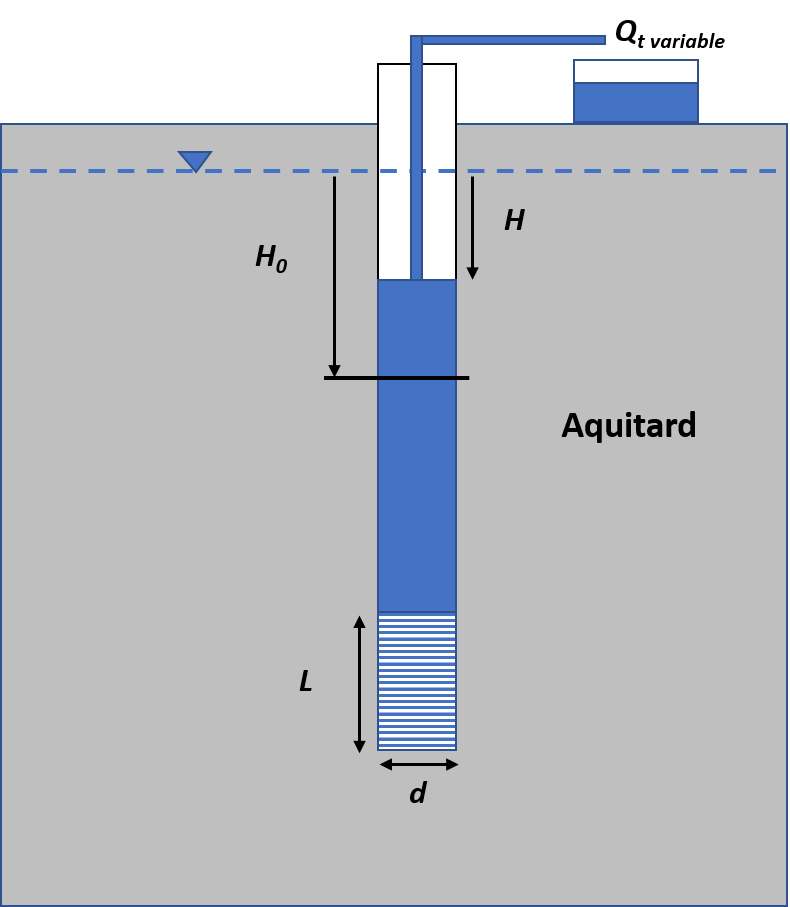
Figure 141 ‑ Slug‑out constant drawdown test set up for a monitoring well. The dashed blue line is the static water level. A slug of water is removed from the well (H0) and at some time during the recovery the unrecovered head, H, in the well is stabilized by extracting volumes of water over time. The test time, t, starts when the variable discharge begins. L is the length of the perforated interval and d is the diameter.
Tavenas and others (1990) developed a method to analyze the data using plots of Q(t) versus 1/t0.5. This relationship should be linear after 5 to 10 minutes from the test initiation. Using an arithmetic plot, a line is fitted to the linear portion of the data and then extrapolated to 1/t0.5 = 0. The steady‑state flow, Qinfinity, is determined by the intersection with the y axis. Using the steady‑state flow rate, Kh is computed as shown in Equation (127).
| [latex]K_{h} = \ \frac{Q_{infinity}}{F\ H}[/latex] | (127) |
|---|
where:
| Kh | = | horizontal hydraulic conductivity (LT‑1) |
|---|---|---|
| Qinfinitity | = | Steady‑state flow rate from graph (L3T‑1) |
| F | = | shape factor for the monitoring well (function of radius, screen length and other factors) (L) |
| H | = | unrecovered head as illustrated in Figure 141 (L) |
The shape factor can be approximated as suggested by Hvorslev (1951) and shown in Equation (128).
| [latex]F\ = \ \frac{2\ \pi\ L}{\ln\left( \frac{L}{d} + \ \left( 1 + \left( \frac{L}{d} \right)^{2} \right)^{.5} \right)}[/latex] | (128) |
|---|
where:
| L | = | perforated length (L) |
|---|---|---|
| d | = | diameter of the perforated interval (L) |
Tavenas and others (1990) provide additional discussion of parameters. The Jacob‑Lohman (1952) solution as outlined by Lohman (1972) may also be applicable for analyzing constant‑head tests. This method assumes a constant head from a flowing well where the change in discharge over time is recorded.
When aquitard material lies at or near the surface, permeability has been investigated using other methods referenced by Cherry and others (2006). These include monitoring and analyzing head changes within the aquitard induced by
- Natural, precipitation‑induced recharge (e.g., Davis, 1972; Keller et al., 1989; Boldt‑Leppin & Hendry, 2003),
- flow into a large, augured cavity (Keller et al., 1989), and
- construction loading and unloading (van der Kamp & Maathuis, 1985).
Aquitard properties can also be estimated based on the calibration of one‑dimensional and three‑dimensional numerical models given hydraulic test data from a site (e.g., Pavelko, 2004; Hart et al., 2005; Anderson et al., 2015).
External Methods
External methods include pumping adjacent water‑bearing units and observing the changes in water levels in the aquitard or in monitoring wells in the pumped aquifer. Examples of these methods are presented in the following subsections.
Pumping Test with An Observation Well in the Aquitard
Neuman and Witherspoon (1972) develop a method to determine the diffusivity, K’/Ss’ (aquitard horizontal hydraulic conductivity and specific storage), when a pumping test is conducted in the underlying or overlying aquifer and a monitoring well or piezometer is installed in the aquitard in concert with a monitoring well in the aquifer as shown in Figure 142. The aquitard well and aquifer‑observation well are at the same radial distance from the pumping well. When an aquifer monitoring well is not present, the drawdown in the pumped aquifer can be projected for the specified radial distance using a Theis analysis of the test data (Neuman & Witherspoon, 1972).
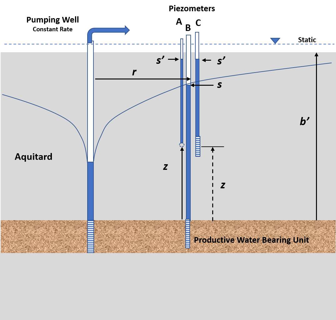
Figure 142 ‑ Schematic of a pumping test conducted in an aquifer and observation wells in that unit (well B) as well as the overlying aquitard (well C). z is the distance from the top of the water bearing unit to the open interval of the observation well in the aquitard. Neuman and Witherspoon (1972) assumed the observation well opening was represented by a point (indicated by A). Rowe and Nadarajah (1993) accounted for the length of well screen where z is the distance from the boundary to the center of the well screen (dashed) (C). The radial distance to the observation well is r. b’ is the thickness of the aquitard unit. At a time after the pumping starts and when drawdown in the aquitard is observed, values of drawdown s’ in the aquitard and s in the unit being pumped (measured from the initial static water level elevation) are recorded.
The method assumes units being pumped and aquitards are infinite in lateral extent and the monitoring wells are located within about 60 m of the pumping well. Detailed observations of drawdown should be collected at early test times. The usable early‑time response of drawdown in the main pumped water‑bearing unit and aquitard are conservatively constrained as indicated by Equation (129).
| [latex]t\ \leq \ 0.1\ \frac{S_{s}'\ {b'}^{2}}{K’}[/latex] | (129) |
|---|
where:
| t | = | the time since the beginning of the pumping (T) |
|---|---|---|
| Ss’ | = | specific storage of the aquitard (L‑1) |
| b’ | = | thickness of the aquitard(L) |
| K’ | = | hydraulic conductivity of the aquitard (isotropic) (LT‑1) |
The time computed by Equation (129) is considered overly conservative (Neuman & Witherspoon, 1969). They suggest that the early‑time limit can be determined by observing when the straight‑line portion of a log‑log time‑drawdown plot for an observation well in the aquitard begins to depart from a linear slope.
At a radial distance (r) and a selected time (t), drawdown (s) is measured in a monitoring well in the water‑bearing unit and drawdown (s’) is measured in a monitoring well or piezometer located in the aquitard. Both wells are located at the same radial distance from the pumping well. Neuman and Witherspoon (1972) assumed that the piezometer in the aquitard is represented as a point (the midpoint of the open interval) and head changes are instantaneous. They developed several curves that relate the drawdown ratio to parameters, tD, and tD’ (Figure 142). As stated previously, additional curves for matching can be generated from the appropriate analytical solution.
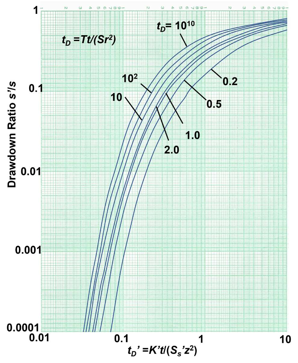
Figure 143 ‑ Neuman and Witherspoon (1972) ratio‑method plots showing the relationship between the drawdown in the pumped unit and an observation well (point source) in an aquitard (s’/s), and factors tD and tD’. tD values between 102 and 1010 are very close together and can be interpolated (modified from Neuman & Witherspoon, 1972; Rowe & Nadarajah, 1993).
| [latex]t_{D} = \frac{Tt}{Sr^{2}}[/latex] | (130) |
|---|
where:
| T | = | pumped unit transmissivity (L2T‑1) |
|---|---|---|
| t | = | time since the pumping began (T) |
| S | = | storativity of the pumped unit (dimensionless) |
| r | = | radial distance to the aquitard piezometer (L) |
and
| [latex]t_{D}' = \frac{K't}{S_{s}z^{2}}[/latex] | (131) |
|---|
where:
| K’ | = | aquitard vertical hydraulic conductivity (LT‑1) |
|---|---|---|
| t | = | time since pumping began (T) |
| Ss’ | = | specific storage of aquitard (L‑1)) |
| z | = | vertical distance from the top of the aquifer to the aquitard piezometer (L) |
When tD is less than 100, estimates of tD’ should use the relationships shown in Figure 143. If tD is greater than 100, multiple curves plot close together and estimated values of tD’ are often determined by using the curve labeled 102. This will yield acceptable results with a small error (e.g., Neuman & Witherspoon, 1972; Rowe & Nadarajah, 1993).
The ratio method requires that the estimates of T and S be computed for the water‑bearing unit being pumped using early‑time data when leakage rates and volumes are low. Often a Theis analysis can be applied.
Ideally, a standard monitoring well is installed in the pumping unit at the same radial distance from the pumping well as the monitoring well in the confining unit. Again, at early‑time, the ratio of drawdown in the aquitard well and aquifer‑monitoring well, s’/s, is computed. The relationships of s’/s and the computed tD value are used to determine a value of tD’ by reading from the x axis of Figure 143. The unknown variable is K’/Ss’. A value of Ss’ is derived from consolidation testing as described in Box 9.3 or the literature as explained in Box 2. Once Ss’ is estimated, a value of K’ is calculated. Neuman and Witherspoon (1972) reported values of K’/Ss’ as representing the portion of the aquitard defined by the distance z (e.g., the portion of the aquitard within the distance z from the aquifer unit which may overlie or underlie the aquitard).
Rowe and Nadarajah (1993) modified Neuman and Witherspoon’s (1972) ratio method by accounting for the perforated length of an aquitard‑monitoring well. This contrasts with the point‑location assumption of Neuman and Witherspoon (1972) as shown in Figure 142. They note that the ratio method used the assumption that the piezometer had an immediate response to pressure change in the aquifer. Rowe and Nadarajah (1993) addressed the effects of using finite‑length perforated intervals in aquitard wells and presented graphics with correction factors for aquitard‑monitoring well‑drawdown data. The measurement location is represented as the midpoint of the screened interval. They also examined the effect of aquitard‑monitoring wells located near the top of the pumping‑unit boundary as expressed in Equation (132). Rowe and Nadarajah (1993) provide more details in their publication.
| [latex]K' = \frac{t_{D}'\ S_{s}'\ z^{2}}{t}\frac{B_{2}^{2}}{B_{1}}[/latex] | (132) |
|---|
where:
| t’D | = | K’t/(Ss’z2) from Figure 1 in Rowe and Nadarajah (1993), which is the same as Figure 142 in this book (L2) |
|---|---|---|
| Ss’ | = | specific storage of aquitard (L‑1) |
| z | = | distance from the aquifer to the midpoint of the piezometer screen in the aquitard (L) |
| t | = | elapsed time since pumping began (T) |
| B1 | = | correction factor for time (Figure 5 in Rowe and Nadarajah, 1993) (dimensionless) |
| B2 | = | correction factors for time (Figure 8 in Rowe and Nadarajah, 1993) (dimensionless) |
Figures for Rowe and Nadarajah (1993) correction factors are reproduced in Box 10 for Groundwater Project readers who do not have access to commercial journals.
In some settings, a number of monitoring wells are placed in an aquitard and the underlying or overlying aquifer is pumped to qualitatively determine if the aquitard is homogeneous or contains heterogeneities such as high‑permeability zones or fractures. Grisak and Cherry (1975) conducted a sequence of pumping tests with wells in an aquifer overlain by a surficial clay‑rich aquitard. Multi‑level monitoring wells were placed in the aquitard. By comparing the rates and magnitudes of responses they interpreted that some wells were finished in blocks of unfractured matrix and others intersected fractures in the aquitard. They then used Hantush analyses of the pumping tests to derive broad‑scale K’ values for the aquitards and finite‑element modeling to adjust estimates of K’ so model results matched observed observation‑well water levels.
Pumping Tests with Observation Wells in Adjacent Productive Units
Pumping tests conducted in productive water‑bearing units confined by aquitards yield information on the hydraulic properties of aquitards. If water‑level responses to pumping mirror the Thesis solution, then the aquitards are acting as impermeable units. In these settings, leakage rates through the aquitard and water released from aquitard storage are sufficiently small and the aquitard is considered impermeable (aquiclude).
In contrast, if aquifer drawdowns reflect the addition of water via the aquitard, then pumping‑test analyses can provide information on the vertical hydraulic conductivity of the aquitard and, in some cases, the storage properties of the adjacent confining unit.
When pumping‑test results match the Hantush‑Jacob or Hantush models for leaky aquifers the general properties of the associated aquitards can be determined as illustrated in Figure 144, which repeats the images of Figure 49 for the readers’ convenience in recalling the groundwater‑system settings. Analysis methods are discussed in Section 9 and are not restated here.
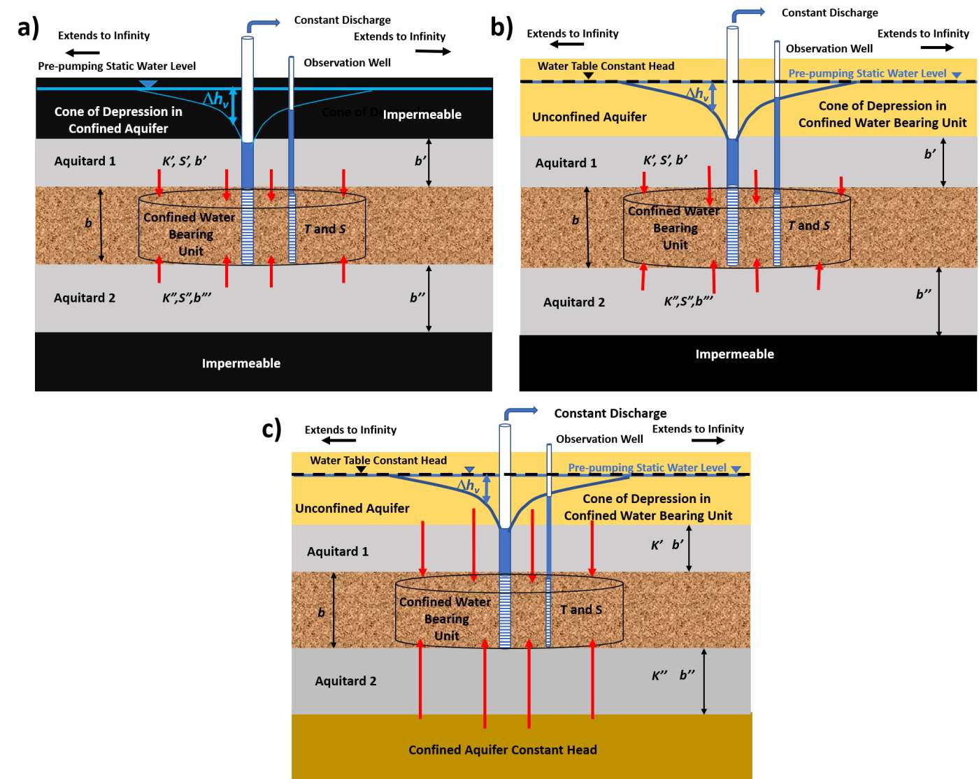
Figure 144 ‑ Standard pumping‑test methods that yield hydrogeologic properties of the confining units that are associated with a confined water‑bearing unit.
a) Drawdown in a confined aquifer that receives water from storage in one or two confining beds when the beds overlying and underlying the confining beds are not permeable.
b) Drawdown in a confined aquifer that receives water from storage in overlying and/or underlying confining beds, as well as leakage of water through the confining bed from a highly transmissive unit such as an unconfined water‑table aquifer.
c) Drawdown in a confined aquifer receiving water via direct flow through a confining bed that has negligible storage from a highly transmissive aquifer above and/or below the confining bed.
Aquitards generally restrict the movement of groundwater and contaminants. When building conceptual models, developing water budgets, mapping flow paths, assessing resident times, and constructing three‑dimensional numerical models, it is as important to establish the properties of aquitards as well as those of aquifers. This section provides basic methods used to characterize aquitards. Additional methods can be found in the literature and the reader is directed to these when assessing more complex settings (e.g., Cherry et al., 2006; Bradbury et al., 2006).