
Solution Exercise 5
A production well was designed to yield 2,000 m3/d from a 40 m thick confined gravel‑rich aquifer. The well was 40 cm in diameter and screened over 35 m. Once the well was completed, a step test was conducted by pumping the well at 1,400 m3/d, 1,790 m3/d and then 2,520 m3/d for a total of 90 minutes with each step lasting 30 min. The time‑drawdown data and a semi‑log plot of the time‑drawdown data are presented here.
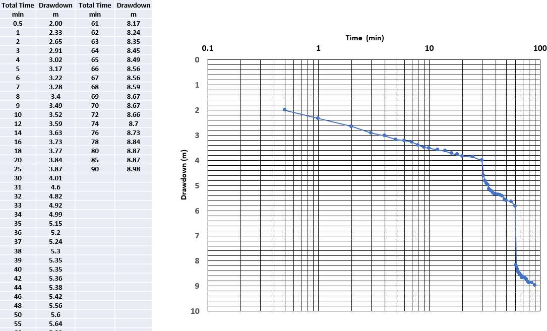
Step‑drawdown test data for a production well. a) Time‑drawdown data for three steps. b) Plot of the log of time versus drawdown.
An Excel® data base of the time‑drawdown data is available on the web page for this book↗.
- Calculate the value of C and B for this system. Compute the well loss expected when pumping the well at 2,000 m3/d.
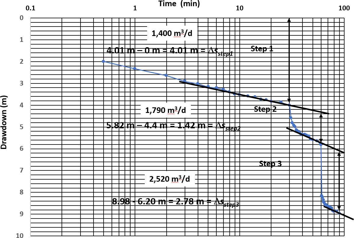
Plot of drawdown versus the log of time showing the calculation of ∆s values. ∆sstep1 for the first 30‑minute step is computed as the difference from the drawdown at zero time and the drawdown at 30 min (double arrow). ∆ sstep2 is computed by subtracting the drawdown at 60 min from the extrapolated drawdown value from the first step (double arrow). ∆sstep3 is computed in a similar fashion from the drawdown at 90 minutes.
A graph of s/QT versus total Q is prepared by computing the ratios of ∆s/Q and Q.
[latex]\frac{\Delta s_{step1}}{Q_{1}} = \frac{4.1\ m}{1400\frac{m^{3}}{d}} = 0.0029\frac{d}{m^{2}}[/latex]
[latex]\frac{\Delta s_{step1} + \Delta s_{step2}}{Q_{2}} = \frac{4.1\ m\ + \ 1.42\ m}{1790\frac{m^{3}}{d}} = 0.003\frac{d}{m^{2}}[/latex]
[latex]\frac{\Delta s_{step1} + \Delta s_{step2} + \Delta s_{step3}}{Q_{3}} = \frac{4.1\ m\ + \ 1.42\ m + 2.78\ m}{2520\frac{m^{3}}{d}} = 0.0033\frac{d}{m^{2}}[/latex]
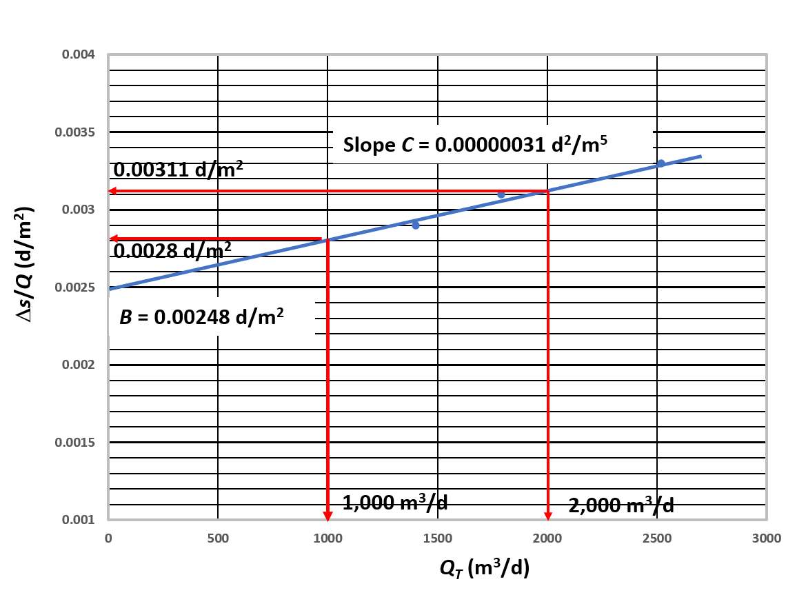
Plot of ∆s/Q versus the log of the corresponding total QT for each step. The slope of the line (C) is computed as the difference in the ∆s/Q values (e.g., horizontal red arrows) divided by the corresponding difference in pumping rate (vertical red arrows).
Reading values to define the slope from the graph, C is determined as follows.
[latex]\begin{aligned} C &= \ \frac{0.0031\frac{d}{m^{2}}\ - \ 0.0028\frac{d}{m^{2}}}{2000\frac{m^{3}}{d}\ - 1000\frac{m^{3}}{d}} \\ &= 0.0000003\ or\ 3x10^{- 7}\frac{d^{2}}{m^{5}} \end{aligned}[/latex]
B is read from the graph as the y‑intercept at QT = 0 as B = 0.00248 d/m2.
The well loss (CQ2) when pumping at 2,000 m3/d would be computed as follows.
[latex]well\ loss = \ 0.0000003\ \ d^{2}/{m\ }^{5}\ \ (2000\ m^{3}/d)^{2}\ \ = \ 1.2\ m[/latex]
- Estimate the total drawdown after pumping the well for 30 min at 2,000 m3/d.
The total drawdown (formational drawdown + well loss) when pumping at 2,000 m3/d for 30 minutes is calculated as follows.
[latex]s_{T} = BQ + CQ^{2}[/latex]
[latex]s_{T} = 0.0028\frac{d}{m^{2}}\left( 2000\frac{m^{3}}{d} \right) + 3x10^{- 7}\frac{d^{2}}{m^{5}}\left( 2000\frac{m^{3}}{d} \right)^{2}[/latex]
[latex]s_{T} = 5.6\ m + 1.2\ m = 6.8\ m[/latex]
To compute total drawdowns at later times new values of B would need to be determined as B is time dependent. This would require inputting a value of T and S in the appropriate equation (e.g., Cooper‑Jacob) and recomputing B for a prescribed period of pumping (t).
- Estimate transmissivity using the first 30 minutes of time‑drawdown data (step 1) (use the Cooper‑Jacob method).
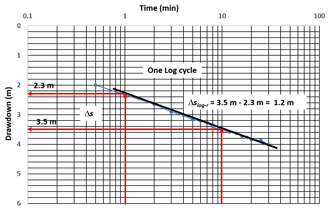
Semi‑log plot of the time drawdown data for step one. A straight‑line fit is performed and a value of ∆slog-t determined. This value is then used in the Cooper‑Jacob analysis to estimate a value of T. As the time drawdown data contains some well loss the storage coefficient is not computed.
The Cooper‑Jacob solution found in Section 8.2.3.
[latex]T = 2.3\frac{Q}{4\pi\Delta s{\Delta s}_{log - t}} = 2.3\frac{1400\ \frac{m^{3}}{d}}{4\ (3.14)\ 1.2\ m} = 214\frac{m^{2}}{d}[/latex]
The time drawdown data in step one has some well loss so T can be determined but S is not estimated as the projected t0 value would be too low (Section 12.1.4). If all the step 1 data were corrected for well loss (sT ‑ CQ2) S could be computed from a semi‑log plot of the corrected data. For example, at 10 min the recorded drawdown is 3.52 m. The corrected drawdown (s) would be as follows.
[latex]s = 3.52\ m - 3x10^{- 7}\frac{d^{2}}{m^{5}}\left( 1400\frac{m^{3}}{d} \right)^{2} = 2.93\ m[/latex]