
Solution Exercise 3
An irrigation well is designed and installed in a 50 m thick highly fractured sandstone that is overlain by 30 m of silt which is in turn overlain by 20 m of sand and gravel. The static water levels in the three units are similar, about 6 m below and surface. The production well is fully penetrating the water producing zone. A 6‑cm diameter, fully penetrating, observation well was constructed in the highly fractured sandstone 23 m from the production well. A 1.9‑day constant rate pumping test was conducted at a rate of 196 m3/d and the observation well water levels were monitored with an electric water level sensor. The test is illustrated in the image shown here.
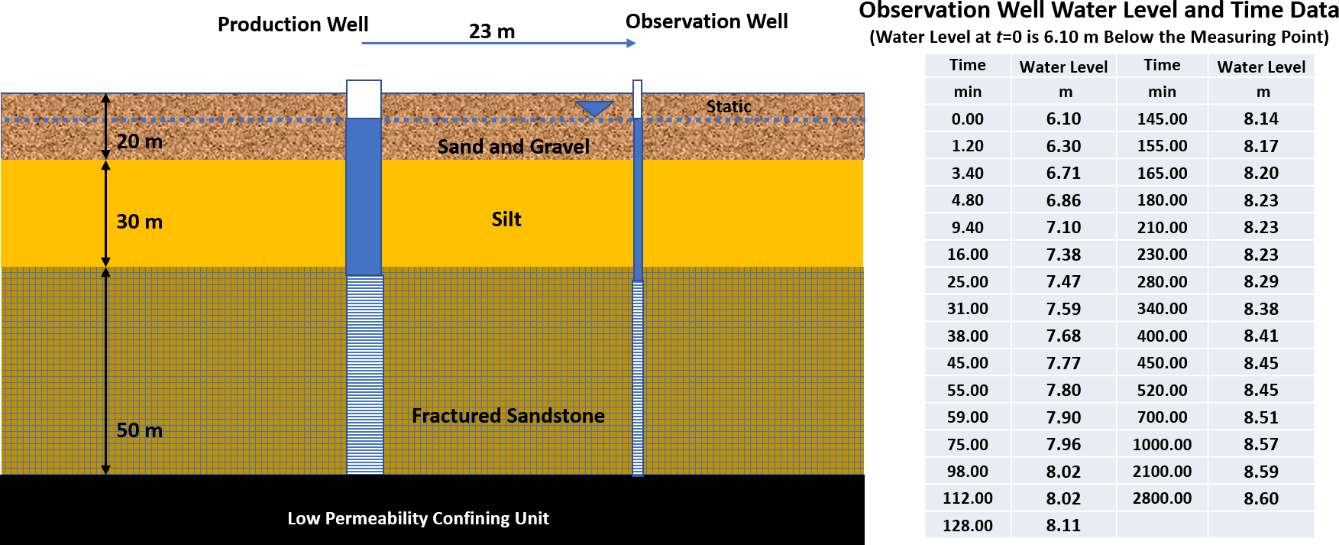
Cross section of hydrogeologic conditions associated with a pumping test. A fractured sandstone is the principal water bearing unit. Static water levels in each unit are about 6 m below land surface. The water level time data collected during the test are shown in the table.
An Excel® data base of the time‑drawdown data is available on the web page for this book↗.
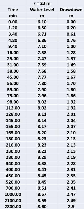
- Convert the water level data to drawdown and plot the data.
Water level data are converted to drawdown as shown here.
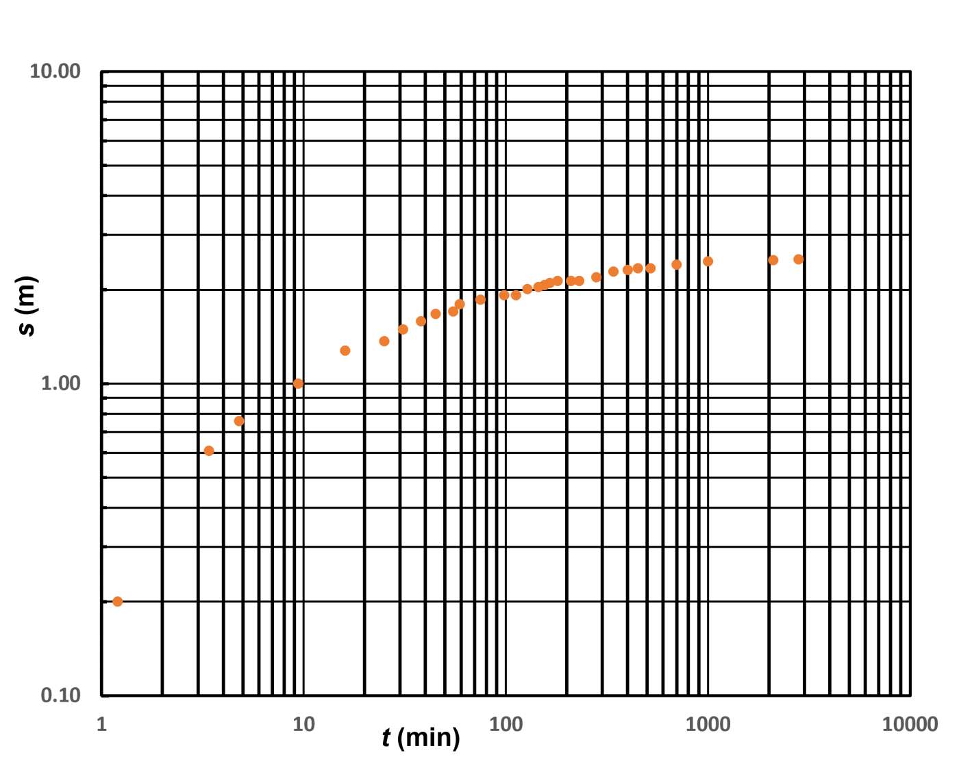
Log‑log plot of drawdown time data (orange dots) for an observation well located 23 m from the pumping well.
- After reviewing the site data, select an analytical approach. Explain why you choose the analytical model used. Treat the highly fractured sandstone as an equivalent porous medium (Woessner & Poeter, 2020). Compute T and S for the highly fractured sandstone aquifer.
The log‑log data plot looks like the response of a totally confined aquifer except it does not match the Theis type curve. The drawdown is behaving as if it is affected by an additional source of recharge, most‑likely from leakage through the silt confining unit. The log‑log plot matches the Hantush‑Jacob family of type curves representing leaky conditions without water released from storage as it appears the drawdown is stabilizing over time.
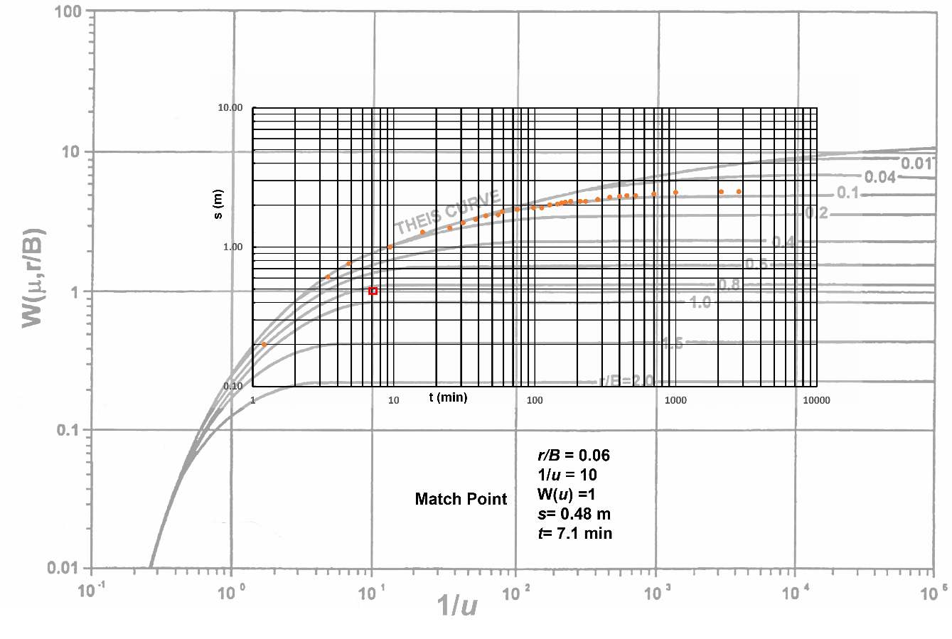
Curve match using Hantush‑Jacob type curves. Time‑drawdown data are represented by orange dots. The match point is indicated by the red rectangle.
A match point is selected as the data appears to mostly fall along the r/B = 0.1 curve.
[latex]T = \frac{Q}{4\pi s}\ W\left( u,\frac{r}{B} \right) = \frac{196\frac{m^{3}}{d}}{4\ (3.14)\ 0.48\ m}(1) = 32.5\ \frac{m^{2}}{d}[/latex]
[latex]S = \frac{u4Tt}{r^{2}} = \frac{(0.1)\ (4)\ 32.5\ \frac{m^{2}}{d}\ 7.1\ min\frac{1\ d}{1440\ min}}{{(23\ m)}^{2}} = 0.00012\ or\ 1.2x10^{- 4}[/latex]
- Based on your analyses, estimate the vertical hydraulic conductivity of the confining silt layer.
Using the match point value of r/B=0.06 then
[latex]K' = \frac{Tb'\left( \frac{r}{B} \right)^{2\ }}{r^{2}} = \frac{32.5\ \frac{m^{2}}{d}(30\ m)(0.06)^{2\ }}{{(23\ m)}^{2}} = 0.0066\frac{m}{d}[/latex]