
Box 2 Estimating Storativity and Specific Storage (Ss)
Saturated geologic materials both transmit and store water. The storage capacity is defined by storativity. Excerpts from Woessner and Poeter (2020) that pertain to defining storativity and specific storage for unconfined and confined water bearing units are reproduced here for the reader’s convenience. Tables of values are also provided in this Box.
Unconfined Aquifer Storativity
The storativity for an unconfined aquifer is dominated by the gravity drainage term, specific yield ([latex]S_{y}[/latex]). Specific yield reflects the volume of water that drains by gravity when the water table is lowered or fills with water when the water table is raised (Figure Box 2‑1). The storativity ([latex]S[/latex]) of an unconfined aquifer is composed of two components as shown in Equation Box 2‑1.
| [latex]S_{unconfined} = S_{y} + S_{s}b_{average}[/latex] | (Box 2‑1) |
|---|
where:
| [latex]S_{unconfined}[/latex] | = | storativity of an unconfined aquifer (dimensionless) |
|---|---|---|
| [latex]S_{y}[/latex] | = | specific yield (dimensionless) |
| [latex]S_{s}[/latex] | = | specific storage (L‑1) |
| [latex]b_{average}[/latex] | = | average thickness before and after a water level change (L) |
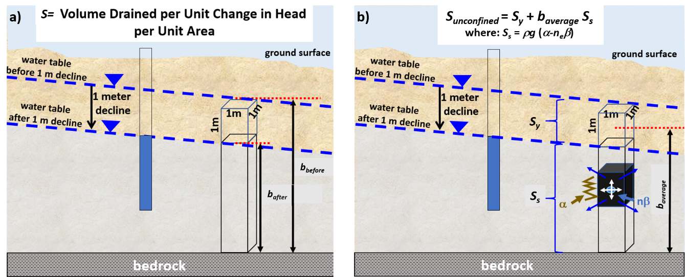
Figure Box 2‑1 ‑ Schematic of components of storativity ([latex]S[/latex]) of an unconfined aquifer. a) Illustration of the definition of the storage coefficient, which is the volume of water released or added to storage per unit change in head normal to the earth’s surface per unit area. b) As the water table is lowered 1 meter, the volume of water released per cubic meter of unconfined aquifer is almost entirely accounted for by water that drains from pores as described by specific yield, [latex]S_{y}[/latex]. The portion of the aquifer that underlies the drained portion also yields a small quantity of water (small blue arrows in black volume) in response to the reduced weight (water drained) of overlying water. The structure of the solids (black volume) compresses (reducing the volume of pore space) as indicated by the compressibility of the aquifer skeleton, [latex]\alpha,\ ([/latex]jagged vertical line). In addition, there is a small expansion of the slightly compressible water, [latex]n\beta[/latex], (blue dot and white arrows). This property of the aquifer is called specific storage, [latex]S_{s}[/latex]. The volume of water released from gravity drainage is orders of magnitude larger than the volume squeezed from the saturated portion of the aquifer, [latex]S_{s}b_{average}[/latex]. As a result, [latex]S_{y}[/latex] is used to represent unconfined aquifer storativity (Woessner & Poeter, 2020; gw-project.org↗).
The specific yield is the volume of water that can drain by gravity from a saturated volume of material divided by the total volume of that material. The fractional volume of water that remains in the sample is called specific retention ([latex]S_{r}[/latex]). It is assumed that, when water is added to storage and the water table rises, the pore spaces that fill already contain only the volume of water indicated by the value of specific retention.
The second term of Equation Box 2‑1 is the product of the specific storage ([latex]S_{s}[/latex]) and the average of saturated thickness before and after drainage ([latex]b_{average}[/latex]). The specific storage is defined as the volume of water that is released from (or added to) storage per unit volume of saturated material. When multiplied by the saturated thickness it accounts for a small amount of water that is released from a unit area of aquifer in response to the relief of stress on the material below the drained pores. It is usually orders of magnitude smaller than the specific yield and is ignored when characterizing storage properties of unconfined systems (Woessner & Poeter, 2020). Table 3 in Woessner and Poeter (2020) is reproduced here to provide estimates of Sy for range of earth materials (Table Box 2‑1).
Table Box 2‑1 ‑ Summary of specific yield values of common earth materials compiled by Morris and Johnson (1967) with additional data from Rivera (2014), Freeze and Cherry (1979), and Domenico and Schwartz (1998) (from Woessner & Poeter, 2020). “NA” represents not available.
| Measurements of Specific Yield for Some Common Earth Materials (Percent) | ||
|---|---|---|
| Material | Number of Samples | Range of Specific Yield Percent |
| Unconsolidated Sediments | ||
| Clay | 27 | 1 ‑ 18 |
| Silt | 299 | 1 ‑ 40 |
| Loess | 5 | 14 ‑ 22 |
| Eolian sand | 14 | 32 ‑ 47 |
| Sand (fine) | 287 | 1 ‑ 46 |
| Sand (medium) | 297 | 16 ‑ 46 |
| Sand (coarse) | 143 | 18 ‑ 43 |
| Gravel (fine) | 33 | 13 ‑ 40 |
| Gravel (medium) | 13 | 17 ‑ 44 |
| Gravel (coarse) | 9 | 13 ‑ 25 |
| Consolidated Sediments | ||
| Shale | NA | 0.5 ‑ 5 |
| Siltstone | 13 | 1 ‑ 33 |
| Sandstone (fine-grained) | 47 | 2 ‑ 40 |
| Sandstone (medium-grained) | 10 | 12 ‑ 41 |
| Limestone and dolomite | 32 | 0 ‑ 36 |
| Karstic limestone | NA | 2 ‑ 15 |
| Igneous and Metamorphic Rocks | ||
| Fresh granite and gneiss | NA | <0.1 |
| Weathered granite/gneiss | NA | 0.5 ‑ 5 |
| Fractured basalt | NA | 2 ‑ 10 |
| Vesicular basalt | NA | 5 ‑ 15 |
| Tuff | 90 | 2 ‑ 47 |
Confined Storativity and Specific Storage
Confined systems remain saturated as the potentiometric surface rises and falls. No gravity drainage occurs. Storativity of a confined system is composed of the water released by the compression and expansion of the unit framework and stored water (Figure Box 2‑2). The following material is reproduced from Woessner and Poeter (2020).
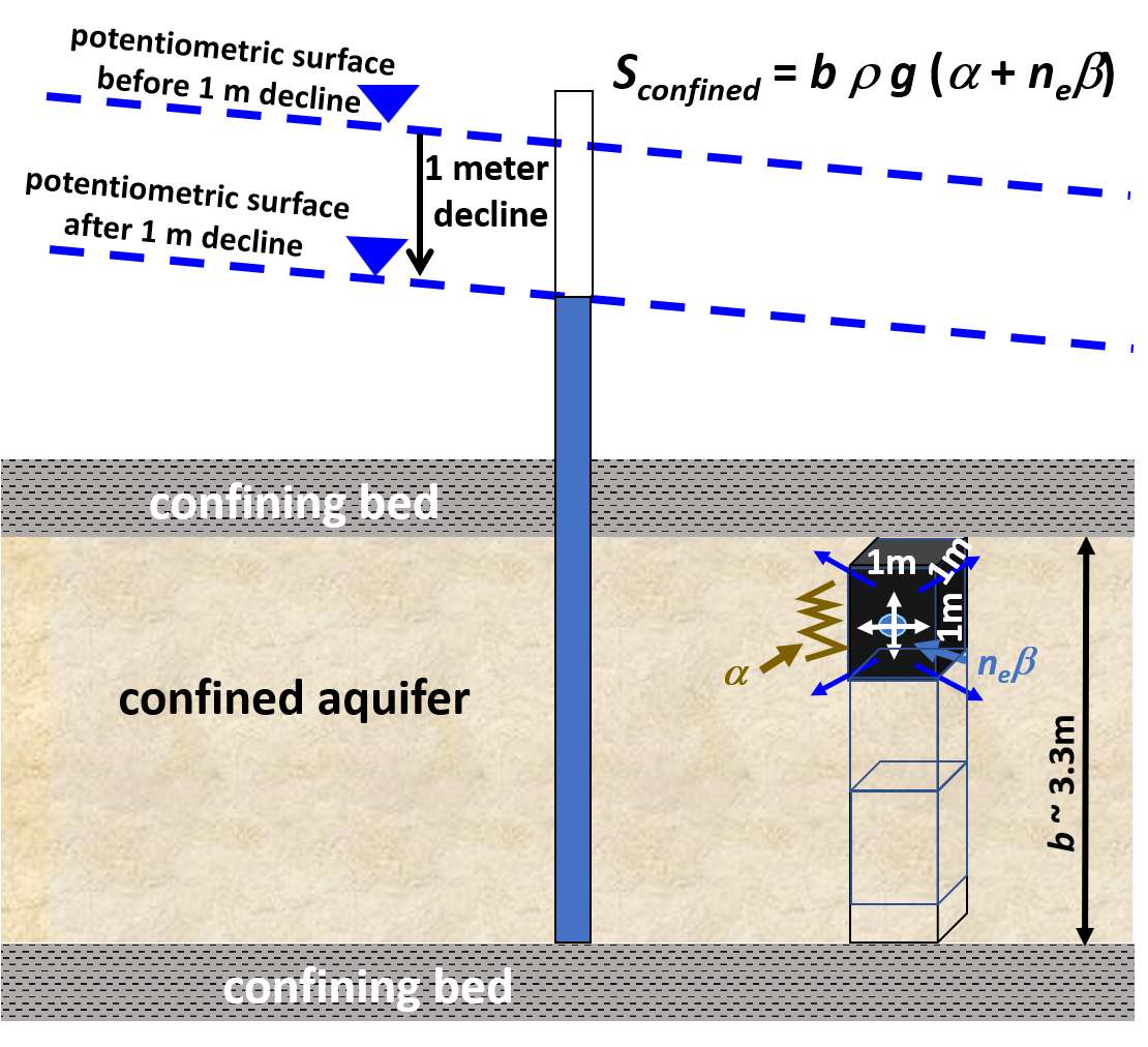
Figure Box 2‑2 ‑ Schematic of the parameters controlling storativity, [latex]S[/latex], of a confined aquifer. The aquifer remains fully saturated as a unit change in the potentiometric surface occurs. Water is released from the entire saturated thickness, [latex]b[/latex], of the aquifer by compression of the skeleton, 𝛼 (jagged line) and expansion of the pore water (blue arrows), [latex]n_{e}\beta[/latex] (Woessner & Poeter, 2020; gw-project.org↗).
When water is released from or added to storage the saturated geologic material either expands or contracts (changes in the effective stress (grain to grain) and/or the water expands or contracts (changes in the pore water pressure). The storativity is defined as representing the volume of water released from or entered storage per unit change in head normal to the surface, per unit area. As the aquifer remains saturated no water gravity drains from the formation.
The confined storativity is defined as the specific storage multiplied by the unit’s saturated thickness (Equation Box 2‑2).
| [latex]S_{confined} = S_{s}b = b\rho g\ \left( \alpha + n_{e}\beta \right)[/latex] | (Box 2‑2) |
|---|
where:
| [latex]S_{confined}[/latex] | = | storativity of an unconfined aquifer (dimensionless) |
|---|---|---|
| [latex]S_{s}[/latex] | = | specific storage (L‑1) |
| [latex]b[/latex] | = | unit saturated thickness (L) |
| d | = | density of water (ML‑3) |
| g | = | acceleration due to gravity (LT‑2) |
| a | = | compressibility of solid matrix (LT2M‑1) |
| ne | = | effective porosity (dimensionless) |
| [latex]\beta[/latex] | = | compressibility of water (LT2M‑1) |
The specific storage, Ss, is defined as the volume of water released from or entered storage per unit change in head normal to the surface, per unit volume of material. The difference in the storativity and specific storage term is that storativity includes the storage properties of the entire thickness of the unit and the specific storage describes the properties of a unit volume of the material.
Computing Specific Storage
Equation Box 2‑3 is used to compute specific storage when values of the compressibility of the materials making up confined system are measured or estimated from literature values.
| [latex]S_{s} = \rho g\ \left( \alpha + n_{e}\beta \right)[/latex] | (Box 2‑3) |
|---|
where:
| [latex]S_{s}[/latex] | = | specific storage (L‑1) |
|---|---|---|
| [latex]\alpha[/latex] | = | compressibility of the material solid structure (LT2M‑1) |
| [latex]n_{e}[/latex] | = | effective porosity (dimensionless) |
| β | = | compressibility of water (LT2M‑1) |
| ρ | = | density of water (ML‑3) |
| g | = | acceleration due to gravity (LT‑2) |
Domenico and Mifflin (1965) presented a table of vertical compressibility, α, for geologic materials. This information can be used with Equation Box 2‑3 to compute specific storage for various confined materials. Dunn (2023) reports that the specific storage values can also be computed assuming water is incompressible (β=0).
Domenico and Mifflin (1965) noted that the specific storage can be approximated by Equations Box 2‑4 through Box 2‑6. Parameters such as vertical compressibility, the bulk modulus of compression, and coefficient of consolidation are derived from laboratory tests or the literature. Box 9 briefly describes laboratory triaxial and consolidation testing methods used to obtain these parameters.
| Ss= (avγw)/(1+e) | (Box 2‑4) |
|---|
where:
| [latex]S_{s}[/latex] | = | specific storage (L‑1) | ||
|---|---|---|---|---|
| [latex]\alpha[/latex] | = | compressibility of the material solid structure (LT2M‑1) | ||
| γw | = | specific weight of water (ML‑2T‑2) | ||
| e | = | void ratio (dimensionless) | ||
| Ss =γw/Ec | (Box 2‑5) | |||
where:
| [latex]S_{s}[/latex] | = | specific storage (L‑1) | ||
|---|---|---|---|---|
| γw | = | specific weight of water (ML‑2T‑2) | ||
| Ec | = | bulk modulus of compression (ML‑1T‑2) | ||
| Ss = Kv/cv | (Box 2‑6) | |||
where:
| [latex]S_{s}[/latex] | = | specific storage (L‑1) |
|---|---|---|
| Kv | = | vertical permeability (LT‑1) |
| cv | = | coefficient of vertical consolidation (L2T‑1) |
We modified Table 1 of Domenico and Mifflin (1965) to report values of specific storage in units of m‑1 (Table Box 2‑2). Two values of specific storage are shown, one computed assuming water is incompressible and the last column accounting for the compressibility of water, γneB, given an assumed porosity value (Woessner & Poeter, 2020). Table Box 2‑2 shows that including the compressibility of water in the calculation of Ss has minimal influence on specific storage values (i.e., differences occur in the 3rd significant figure and beyond). Dunn (2023) also provides a good discussion of specific storage (https://www.dunnhydrogeo.com/home/aquifer-storativity-t↗).
Table Box 2‑2 Material properties including, geologic unit skeletal compressibility (α), assumed values of effective porosity (ne), an assumed value for the specific weight of water γ as 9,810 kgm‑2s‑2, and calculated values of Ss with and without consideration of the compressibility of water (β = 4.3×10‑10 ms2kg‑1). Porosity values are based on material type and have little effect on the calculation of Ss due to the low compressibility of water (modified from Domenico & Mifflin (1965) and Dunn (2023) at the website: https://www.dunnhydrogeo.com/home/aquifer-storativity-t↗).
| Material | α range | Ss = γα | Assumed ne | Ss = γ(α+neβ) |
|---|---|---|---|---|
| ms2kg‑1 | m‑1 | dimensionless | m‑1 | |
| Plastic Clay | 2.0×10‑6 | 1.96×10‑2 | 0.6 | 1.96×10‑2 |
| 2.5×10‑7 | 2.45×10‑3 | 0.6 | 2.46×10‑3 | |
| Stiff Clay | 2.5×10‑7 | 2.45×10‑3 | 0.5 | 2.45×10‑3 |
| 1.3×10‑7 | 1.28×10‑3 | 0.5 | 1.28×10‑3 | |
| Medium Hard Clay | 1.3×10‑7 | 1.28×10‑3 | 0.4 | 1.28×10‑3 |
| 6.8×10‑8 | 6.67×10‑4 | 0.4 | 6.69×10‑4 | |
| Loose Sand | 1.0×10‑7 | 9.81×10‑4 | 0.35 | 9.82×10‑4 |
| 5.1×10‑8 | 5.00×10‑4 | 0.35 | 5.02×10‑4 | |
| Dense Sand | 2.0×10‑8 | 1.96×10‑4 | 0.3 | 1.97×10‑4 |
| 1.3×10‑8 | 1.28×10‑4 | 0.3 | 1.29×10‑4 | |
| Dense Sandy Gravel | 1.0×10‑8 | 9.81×10‑5 | 0.15 | 9.87×10‑5 |
| 5.1×10‑9 | 5.00×10‑5 | 0.15 | 5.07×10‑5 | |
| Rock fissured/jointed | 6.8×10‑9 | 6.67×10‑5 | 0.01 | 6.68×10‑5 |
| 3.3×10‑10 | 3.24×10‑6 | 0.01 | 3.28×10‑6 | |
| Rock sound | 3.3×10‑10 | 3.24×10‑6 | 0.0001 | 3.24×10‑6 |
Another common method used to estimate S for confined aquifers was proposed by Lohman (1972). He noted that storativity of confined aquifers typically range from 0.00001 to 0.001 (1x[latex]10^{- 5}[/latex] to 1x[latex]10^{- 3}[/latex]). He suggests the storativity for a confined aquifer can be approximated as 0.000003/m times the aquifer thickness in meters. This approximation basically results in using 0.000003/m as an estimate of the specific storage for all confined earth materials. Using his approach, estimated storativity values are in the 10‑5 to 10‑4 range when the thickness of rock based confined systems are 10’s to 100’s of meters. Lohman’s (1972) approach provides a poor estimate of specific storage when aquifer or aquitard materials are something other than hard rock. Thus, specific storage estimates based on Table Box 2‑2 should be used with aquifer thicknesses to estimate storativity values for confined systems when pumping test computed values are not available.