
12.1 Special Considerations When Using Drawdown Data from a Pumping Well
Under ideal conditions, analytical solutions (Sections 7 through 10) and their simplifying assumptions can be applied to single‑well pumping‑test data to determine corresponding values of T and S. However, wells need to be fully penetrating and 100 % efficient. When using drawdown in the pumping well for the analysis, the pumping well radius is often substituted in the equations that require a radial distance to an observation well. The screen or perforated‑casing radius is used unless the well construction includes an envelope of gravel pack. When this occurs, the well radius is defined as the effective well radius and includes the radius of the perforated interval and gravel pack.
However, when a single pumping well is the only source of drawdown data, it must be recognized that the recorded drawdown data are often influenced by partial penetration, well‑bore storage, and well loss, which are functions of the well design. Partial‑penetration and well‑loss effects result in lower water levels in the pumping well as compared to the adjacent aquifer. Well‑bore‑storage effects temporarily reduce the rate of early water level decline when large diameter wells are pumping at low rates. Each of these conditions are usually present to some degree and directly affect the predicted or reported drawdown at the pumping well. As with observation well test records, pumping‑well drawdowns can be impacted by well interference, barometric, tidal, and, in unconfined cases, recharge events and direct evapotranspiration.
Most often partial penetration and well‑loss conditions result in greater drawdown measured in the pumping well than if they were not present. As a result, computed T and S values are lower than properties of the formation. Ideally, pumping‑well drawdown would be corrected before analyses were undertaken.
During the early‑time period of some pumping tests—especially in large‑diameter wells—pumped water is derived not only from the aquifer but also from water stored in the well casing or annular space (and filter pack) surrounding the screened or perforated interval. This results in a reduction in the observed drawdown in the pumping well and is referred to as a wellbore storage effect. As time progresses, formational water makes up an increasing portion of the well discharge until wellbore storage effects are sufficiently small, and flow is supplied by the aquifer. The influence of wellbore storage on drawdown data is most easily observed using log‑log plots of time‑drawdown data. The early‑time data will appear as a straight line diverging from the Theis curve. Papadopulos and Cooper (1967) developed an analytical method and a set of type curves that can be used to analyze confined‑aquifer‑test data affected by wellbore storage. Moench (1997) generated an analytical solution for pumping unconfined aquifers that accounts for well bore storage. He also provides a set of type curves.
The total observed pumping‑well drawdown can be visualized as having several components as shown in Figure 79 and explained by Equation (79).
| [latex]s_{T} = s_{F\ } + s_{pp\ } + s_{WL\ } + s_{I\ } + s_{O\ }[/latex] | (79) |
|---|
where:
| sT | = | total observed drawdown in the pumping well (L) |
|---|---|---|
| sF | = | component of drawdown based solely on the formational properties (T, S) (L) |
| spp | = | component of drawdown resulting from partial penetration of the perforated interval (L) |
| sWL | = | component of drawdown from linear and non‑linear well loss (L) |
| sI | = | component of drawdown from well interference (L) |
| sO | = | component of drawdown from other factors with a positive or negative sign (e.g., wellbore storage, barometric effects, tides, recharge) (L) |
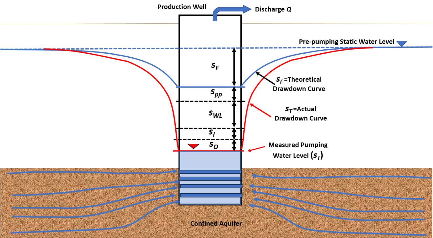
Figure 79 ‑ Schematic of a partially penetrating pumping well in a confined aquifer (sand pattern) showing components of the total drawdown (sT) as represented by the red profile. The formational drawdown (sF) is shown in the blue drawdown profile and is the drawdown if the well is 100 percent efficient and fully penetrating. Additional components contributing to the total drawdown observed in the pumping well may include the effects of partial penetration which results in longer flow paths to the well as indicate by the blue flow lines (spp), well loss resulting from the well construction, design, and pumping rate (sWL), drawdown from wells pumping nearby which is called well interference (sI), and other factors causing the water levels to rise or fall such as wellbore storage and barometric effects (s0).
The measured water levels in the pumping well will be similar to the theoretical drawdown shown in blue on Figure 79 if:
- the pumping well is fully penetrating and 100 percent efficient,
- wellbore storage has been depleted
- there are no head losses due to turbulent flow caused by high flow rates and/or obstructions in the well, and
- there is no interference from nearby pumping wells or other hydraulic stresses on the unit being tested.
The following sections describe how the factors that require special consideration influence drawdown data in the pumping well and present methods used to quantify the magnitude of their effect and to correct the drawdown data.
Partial Penetration
A partially penetrating pumping well produces vertical components of flow near the well in both confined and unconfined aquifers. The vertical flow component creates longer flow paths that result in the flow system expending more energy to deliver water to the well than if all flow is horizontal. Partial‑penetration effects can occur in an unconfined aquifer as pumping begins even if a well is fully penetrating when the saturated thickness adjacent to the pumping well is reduced significantly during the test.
Todd and Mays (2005) provide methods to compute the increase in drawdown attributed to the head loss during groundwater flow to a partially penetrating well. They report that if the perforated interval of the well penetrates 85 percent or more of the aquifer then correction is not necessary, but it is generally accepted that correction is not necessary if the screened portion of a well penetrates 80 percent or more of the aquifer thickness.
When considering the effects of partial penetration only, the total drawdown is composed of the formational drawdown, sF, and the additional drawdown ∆spp caused by partial penetration as shown in Equation (80) and Figure 80.
| [latex]s_{T} = s_{F} + \mathrm{\Delta}s_{pp}[/latex] | (80) |
|---|
where:
| sT | = | total drawdown in pumping well including effects of partial penetration and formational drawdown (L) |
|---|---|---|
| sF | = | formational drawdown (L) |
| ∆spp | = | drawdown due to partial penetration (L) |
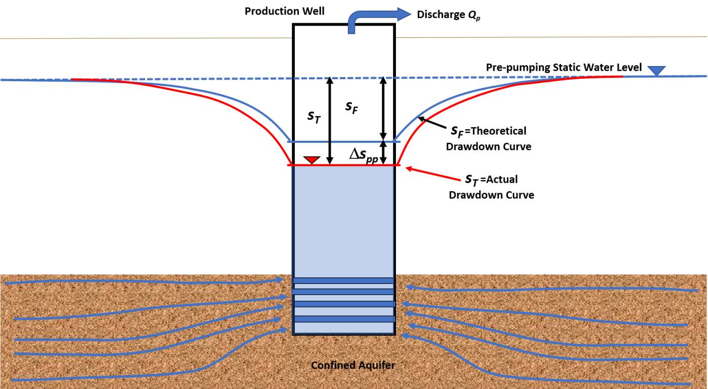
Figure 80 ‑ Total drawdown, sT, associated with a partially penetrating pumping well when both formational drawdown, sF, and drawdown related to the effects of partial penetration, ∆spp occur.
Huisman (1972) and Todd and Mays (2005) present methods to compute the effects of partial penetration using steady‑state formulations, the variables shown in Figure 80 and Figure 81, and a penetration factor p = hs/b, screen length (hs) divided by the saturated aquifer thickness (b).
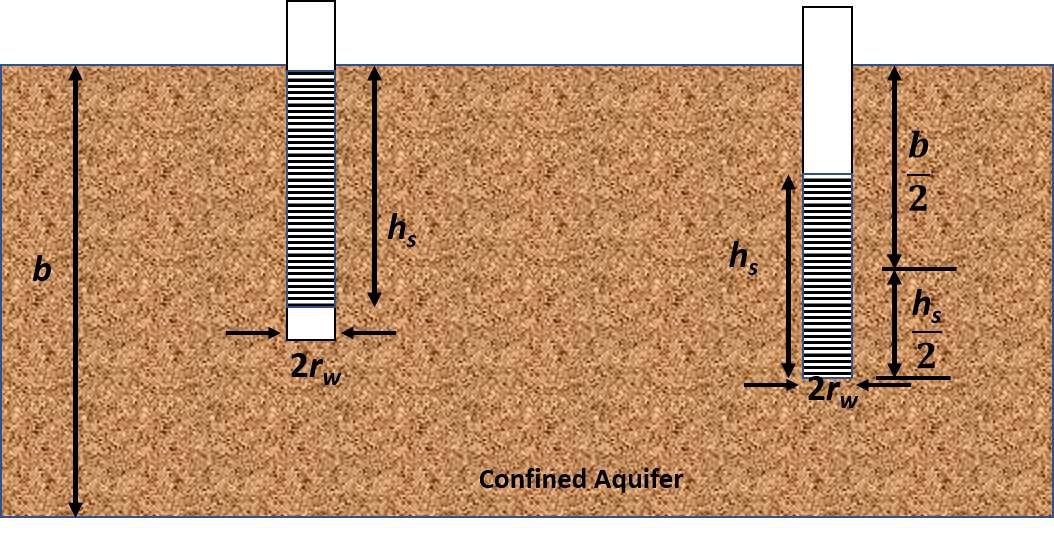
Figure 81 ‑ Schematic of a confined aquifer (sand pattern) and the perforated interval (horizontal black lines) for two production wells. b represents the initial saturated thickness of the aquifer. hs is the length of the perforated interval and rw is the radius of the well (after Todd & Mays, 2005).
The additional drawdown associated with partial penetration under steady‑state conditions in a confined aquifer as represented on the left‑hand side of Figure 80 is defined for p > 0.2 by Todd & Mays (2003) in Equation (81). When the well screen is centered in the formation as shown in the right‑hand portion of Figure 81, then p = (hs/2)/(b/2) and this ratio is substituted into Equation (81) that becomes Equation (82).
| [latex]\mathrm{\Delta}s_{pp} = \frac{Q_{p}}{(2\pi T)}\left( \frac{1 - p}{p} \right)\ln\left( \frac{(1 - p)h_{s}}{r_{w}} \right)[/latex] | (81) |
|---|
| [latex]\mathrm{\Delta}s_{pp} = \frac{Q_{p}}{(2\pi T)}\left( \frac{1 - p}{p} \right)\ln\left( \frac{(1 - p)h_{s}}{2r_{w}} \right)[/latex] | (82) |
where:
| ∆spp | = | additional drawdown resulting from partial penetration (L) |
|---|---|---|
| Qp | = | partially penetrating well pumping rate (L3T‑1) |
| T | = | transmissivity (L2T‑1) |
| p | = | penetration factor, hs/b (dimensionless) |
| hs | = | length of well screen (L) |
| b | = | saturated thickness of aquifer (L) |
| rw | = | radius of the pumping well (L) |
Based on the Thiem equation for unconfined aquifers, the drawdown resulting from partial penetration is defined by Todd and Mays (2005) as shown in Equation (85).
| [latex]\mathrm{\Delta}s_{pp}2h_{w} = \frac{Q_{p}}{(\pi K)}\left( \frac{1 - p}{p} \right)\ln\frac{\left( (1 - p)h_{s} \right)}{r_{w}}[/latex] | (83) |
|---|
where:
| ∆spp | = | drawdown resulting from partial penetration (L) |
|---|---|---|
| hw | = | saturated thickness of the unconfined aquifer at pre‑pumping conditions (L) |
| Qp | = | partially penetrating well pumping rate (L3T‑1) |
| K | = | hydraulic conductivity (LT‑1) |
| p | = | penetration factor p = hs/b (dimensionless) |
| hs | = | length of well screen (L) |
| rw | = | radius of the pumping well (L) |
The total drawdown in an unconfined aquifer is defined as shown in Equation (84).
| [latex]s_{T} = \sqrt{s_{F}^{2} + \mathrm{\Delta}s_{pp}2h_{w}}[/latex] | (84) |
|---|
where:
| sT | = | total drawdown in pumping well including effects of partial penetration and formational drawdown (L) | |
|---|---|---|---|
| sF | = | formational drawdown (L) | |
| ∆spp | = | drawdown from partial penetration (L) | |
| hw | = | saturated thickness of the unconfined aquifer at a fully penetrating well (L) |
The partial‑penetration conditions that cause the additional drawdown are conceptualized as being constant once pumping begins. The partial‑penetration correction can be applied to transient or steady‑state drawdown data.
Example
A well with a radius of 0.15 m finished in a confined unit is pumped at a continuous rate of 4000 m3/d to near steady state and the total drawdown is 34 m. The screened interval is 10 m in length, and it is located just below the upper boundary of a 45 m thick aquifer. If the aquifer transmissivity is 940 m2/d, how much of the drawdown is due to partial penetration?
The penetration factor is 10 m/45 m = 0.22. Using Equation (81), ∆spp is computed as shown here.
[latex]\mathrm{\Delta}s_{pp} = \frac{Q_{p}}{(2\pi T)}\left( \frac{1 - p}{p} \right)\ln\frac{\left( (1 - p)h_{s} \right)}{r_{w}}[/latex]
[latex]\mathrm{\Delta}s_{pp} = \frac{4000\frac{m^{3}}{d}}{2\ (3.14)\ 940\frac{m^{2}}{d}}\frac{1 - (0.22)}{(0.22)}\ln\frac{\left( (1 - 0.22)10\ m \right)}{0.15\ m} = 9.5\ m[/latex]
If a total observed drawdown in the partially penetrating well bore is 26.01 m, then rearranging Equation (80) the formational drawdown would be defined as sF = sT ‑ ∆spp, so sF = 26.01 m ‑9.5 m = 16.51 m. If time‑drawdown data were collected during a transient test, drawdown would be corrected by ‑9.5m.
In addition to the equations presented above, other authors have addressed methods to assess partial penetration effects with analytical solutions for steady‑state and transient conditions (e.g., Sternberg, 1973; Brons & Marting, 1961; Bradbury & Rothschild (1985); Hantush, 1966; Neuman, 1975; Kipp 1973). Most commercial hydraulic‑test‑analysis software packages incorporate methods to correct data for partial penetration once well construction data are entered.
Well Loss and Using Step‑Drawdown Tests to Assess Loss
Well loss is the component of the total drawdown in a production well due to the loss of energy resulting from turbulent flow of water through the screened or slotted interval (or the damaged borehole wall), as well as flow inside the casing to the pump intake as shown in Figure 82 and expressed by Equation (85).
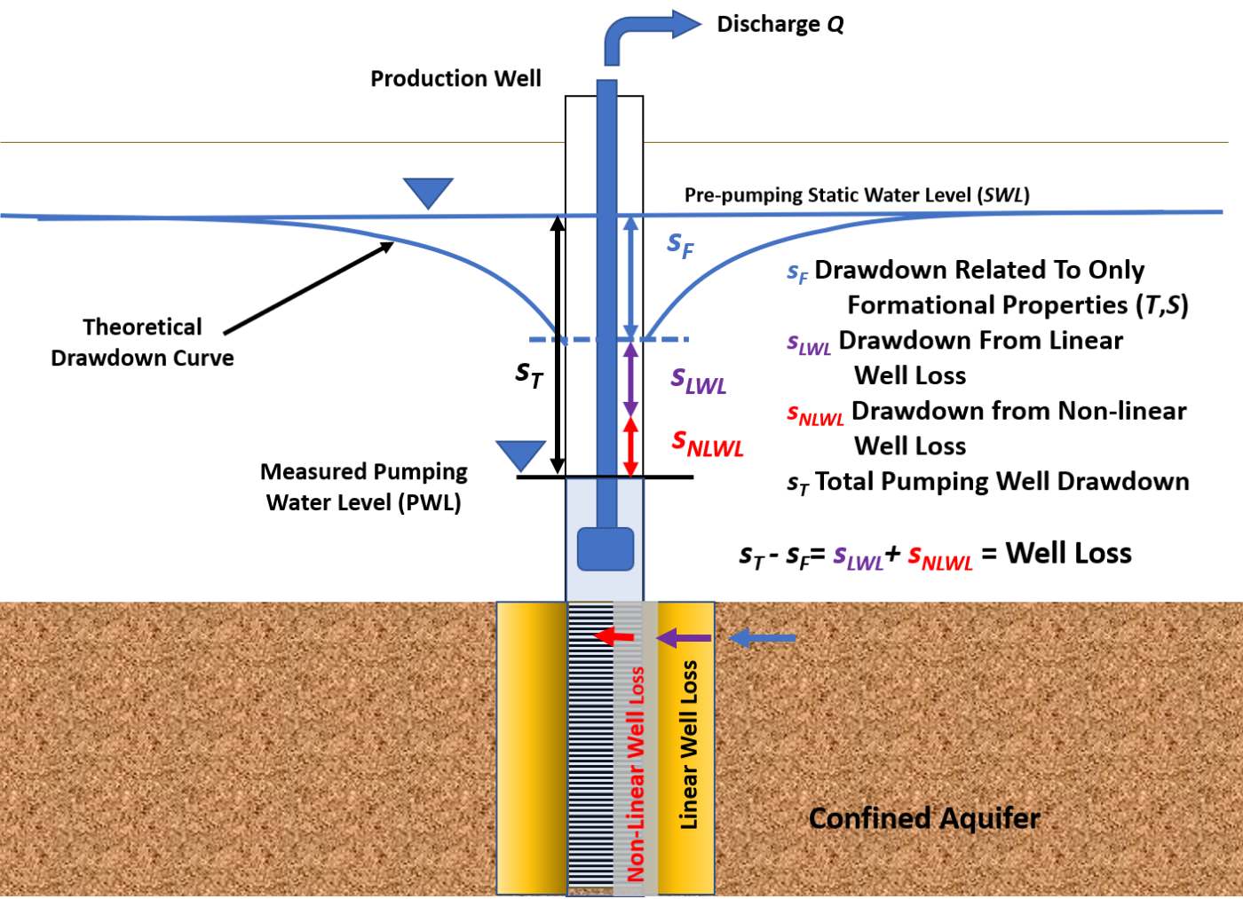
Figure 82 ‑ Schematic showing the components of well loss in a fully penetrating pumping well finished in an isotropic and homogeneous confined aquifer. The measured drawdown is greater than if the well was 100 percent efficient and only the formational drawdown occurred as shown with the theoretical drawdown curve (sF). The well loss is conceptualized as having two drawdown components, linear well loss (sLWL), and non‑linear well loss (sNLWL). As water in the vicinity of the wellbore converges to the perforated interval, head loss occurs as it passes through the area around the well that was impacted by well construction (linear well loss). Head loss also occurs as water moves through the perforations and up the well bore to the pump (non‑linear well loss).
| [latex]s_{WL} = s_{LWL\ } + s_{NLWL}[/latex] | (85) |
|---|
where:
| sWL | = | total well loss (L) |
|---|---|---|
| sLWL | = | linear well loss (L) |
| sNLWL | = | non‑linear well loss (L) |
When additional drawdown in a pumping well occurs from well loss, the total drawdown in the pumping well is the drawdown occurring due to the transmission and storage properties of the formation, sF, and the total well loss (sWL) as expressed in Equation (86).
| [latex]s_{T} = s_{F} + s_{WL}[/latex] | (86) |
|---|
where:
| sT | = | total drawdown (L) |
|---|---|---|
| sF | = | formational drawdown (L) |
| sWL | = | total well loss drawdown (L) |
Hydraulic gradients near the well bore are often affected by formational damage caused by well construction. These include zones of lower hydraulic conductivity (introduction of well cuttings and drilling fluids) that are present adjacent to the well borehole called skin effects (e.g., Sterrett, 2007). As the converging flow enters this area, gradients increase and additional head loss (linear well loss [sLWL]) occurs. These are termed linear losses because their magnitude is directly proportional to the well‑discharge rate. Sometimes the damage zone has less resistance to flow because of performed well development and/or pumping that mobilize fines in the formation, drawing them into the well and enhancing formation conductivity near the well such that sLWL can be negative (Sterrett, 2007). The second component of head loss occurs as flow passes through the perforated interval (screen openings or cut slots) and moves up the well bore to the pump. This reduction in the total head is referred to as non‑linear well loss (sNLHL). These are termed non‑linear losses because their magnitude increases nonlinearly as well discharge increases. Figure 83 illustrates the impact of these loses on drawdown.
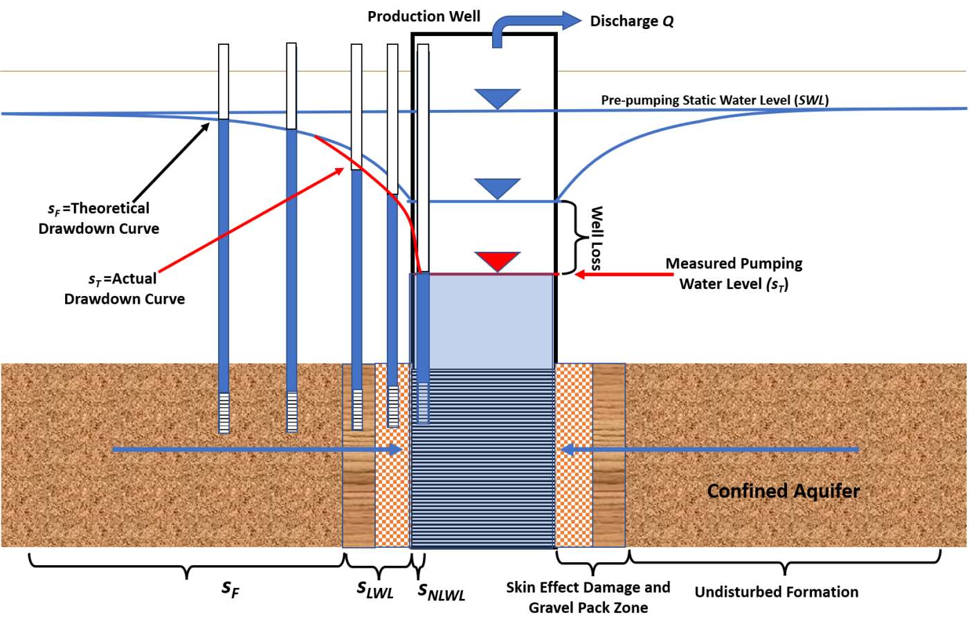
Figure 83 – Schematic of the change in water levels as water flows to the fully penetrating well bore completed in an isotropic and homogeneous confined aquifer being pumped at a constant rate (sand pattern). The small diameter wells (imaginary) are included in the diagram to illustrate the effect of well loss. The blue profile shows the theoretical drawdown (sF) derived when the well has zero well loss (100 percent efficient). The red profile is created by adding the effects of well loss (sLWL+sNLWL) (red line). Zones of formational, linear, and non‑linear well loss are illustrated at the base of the diagram.
Well loss is a function of the flow rate, being larger at higher pumping rates as shown in Equation (87).
| [latex]s_{T} = B_{1}Q + B_{2}Q + CQ^{2}[/latex] | (87) |
|---|
where:
| sT | = | total drawdown (L) |
|---|---|---|
| B1 | = | formational aquifer properties (TL‑2) |
| Q | = | well discharge (L3T‑1) |
| B2 | = | formational conditions for linear well loss (TL‑2) |
| C | = | coefficient representing a non‑linear well loss coefficient (T2L‑5) |
In Equation (87), B1Q=sF, B2Q=sLWL, and CQ2=sNLWL. The values of B1 and B2 are not separable when time‑drawdown data are available for only the pumping well. Jacob (1947) developed a relationship between the value BQ representing the formational drawdown and the non‑linear or turbulent well loss component, CQ2 (Equation (88)). B in this relationship can be conceptualized as B1+B2. For a confined aquifer, B can be calculated using the Cooper‑Jacob transient approximation in which the linear well loss component is formally included. That is, B equals [latex]\frac{1}{4\pi T}\ \ln\left\{ \frac{Tt}{{1.78r}^{2}S} \right\},[/latex] as shown in Equation (31) of Section 8.3.2. Rorabaugh (1953) suggests that the commonly used squared term on C in the non‑linear well loss term can be replaced with a variable that is near two but can be less or greater than two. Rorabaugh (1953) provides additional information. Traditionally, a value of two is assumed.
| [latex]s_{T} = BQ + CQ^{2}[/latex] | (88) |
|---|
where:
| sT | = | total drawdown in the pumping well (L) |
|---|---|---|
| B | = | represents formational aquifer properties (TL‑2) |
| Q | = | well discharge (L3T‑1) |
| C | = | coefficient representing non‑linear well loss (T2L‑5) |
When T and S are known, Equation (88) is used to correct pumping well drawdown for non‑linear well loss by computing CQ2 and subtracting it from the observed drawdown, sF = sT‑CQ2. Step‑drawdown tests are used to estimate the well loss coefficient C.
Step‑Drawdown Test and Methods to Compute Well Loss Coefficient and Estimate T
A step‑drawdown test (often referred to as a step test) is conducted by pumping a well at various rates and recording time‑drawdown data in the well. These tests can be used to investigate the drawdown response to pumping when flow rates increase and decrease. Step‑drawdown testing is used to characterize the well loss that occurs at various pumping rates. This methodology is most often used to quantify the well‑loss coefficient, C. The coefficient is used to compute well‑loss components of the total drawdown at a prescribed pumping rate and to correct drawdown versus time data to reflect drawdown attributed only to formational properties and conditions.
During a step‑drawdown test, the pumping rate is increased from an initially low constant rate through a series of sequentially higher constant pumping rates (steps). Typically, each step is of equal duration, lasting from approximately 30 minutes to 2 hours (Kruseman & de Ridder, 2000). Each step should be of sufficient duration to allow the dissipation of wellbore storage effects. Any number of steps can be conducted; however, at least three are recommended. The steps are usually increased sequentially but can be started and stopped allowing full recovery (Figure 84). The step test is usually designed so that the stepped pumping rates include or bracket the desired pumping rate for a production well. This allows computation of the well‑loss coefficient at that planned pumping rate. Step tests are also used to evaluate well performance including selecting pumping rates with lower well loss and identifying whether well conditions have changed over time (Sterrett, 2007).
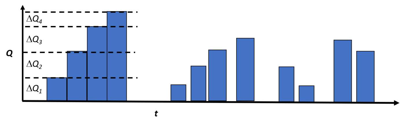
Figure 84 ‑ Step‑drawdown tests are most often conducted as one continuous test where the pumping rate is held constant for a period and then increased by a value of ΔQ as shown in the left‑hand portion of the graph. The length of time each step is pumped, and the ΔQ can vary. Time‑drawdown data are collected for each step. A second approach, shown in the middle and right‑hand side of the diagram, illustrates that step test data sets can also be derived when a well is pumped at a constant rate, then the pumping is stopped, and the well is allowed to recover. Repeating this method for various pumping rates creates a step test data set.
Step‑drawdown test results are plotted on a semi‑log scale as drawdown versus time. The change in drawdown between each step is designated as ∆sstep and the change in discharge between each step is defined as ∆Q. Figure 85 shows data from a continuous step test where each step reached steady‑state drawdown or near steady‑state. Figure 86 shows a transient step test where each step lasted 30 minutes or more and drawdown was still declining as the next step started. In this case, ∆sstep is the difference between the straight‑line projection of the drawdown of the previous step and the drawdown after 30 minutes of pumping at the new rate.
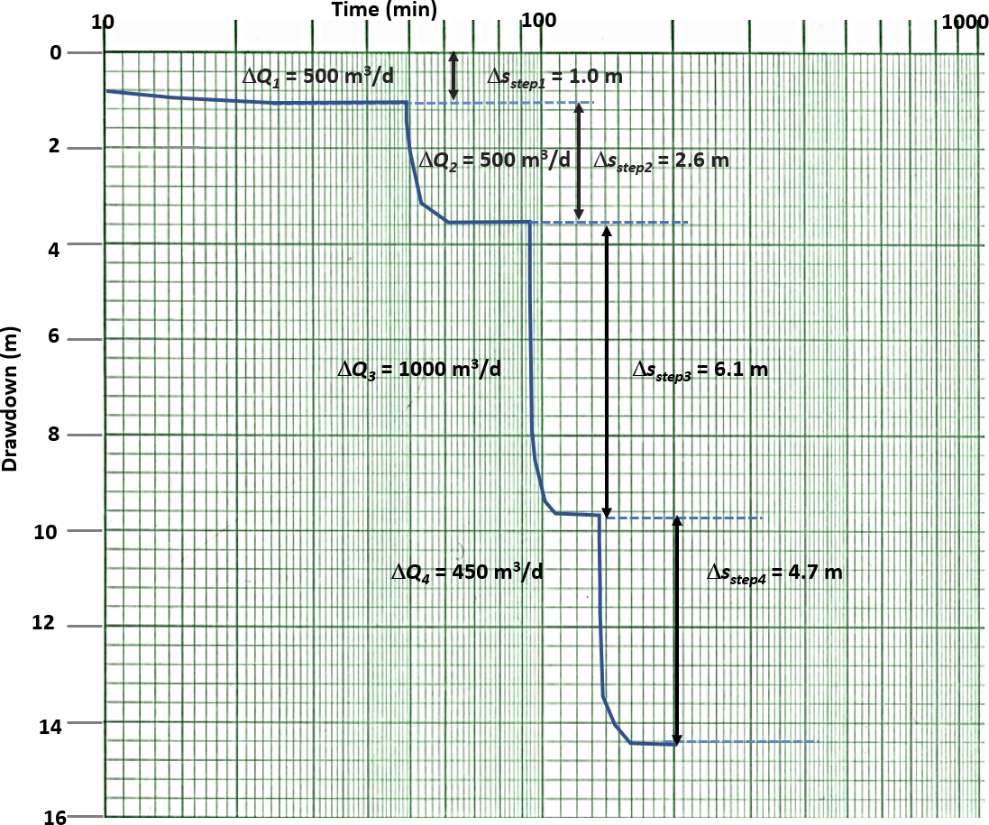
Figure 85 ‑ Step‑drawdown test where sequential constant pumping rates were used, and the drawdown reached steady‑state at each step. Dashed lines represent an extension of the observed drawdown trend. Values of ∆Q and Δsstep are shown. Total pumping rates and drawdown for an individual step are obtained by adding the change in pumping rate and additional drawdown to those of the previous steps.
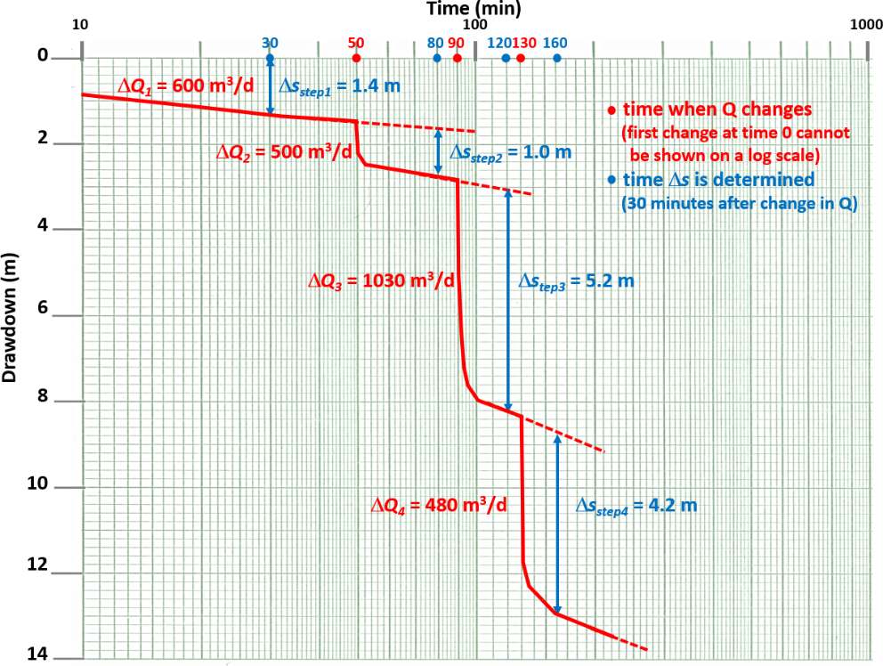
Figure 86 ‑ Transient step‑drawdown test with sequential constant rates. Pumping of each step equaled or exceeded 30 minutes. Dashed lines represent extensions of the observed drawdown trends. Using a 30‑minute interval from the start of each step, values of ΔQ and Δsstep are shown. Total pumping rates and drawdown for each step (after 30 minutes of pumping) are obtained by adding the changes in pumping rates and drawdown up to that point (i.e., ΣΔQ and ΣΔsstep).
Analysis of the steady‑state step‑drawdown test shown in Figure 85 is described next. To estimate the turbulent flow coefficient, C, and the formational coefficient, B, of Equation (88), an arithmetic plot of the total discharge for each step and the total drawdown divided by the total step discharge for each step (s/QT) is plotted (Figure 87). QT is the cumulative pumping rate for a step, e.g., QT for step 2 is ∆Q1+∆Q2, and for step 3 QT = ∆Q1+∆Q2 +∆Q3. This approach is referred to as the Hantush‑Bierschenk method (Hantush, 1964; Bierschenk, 1963).
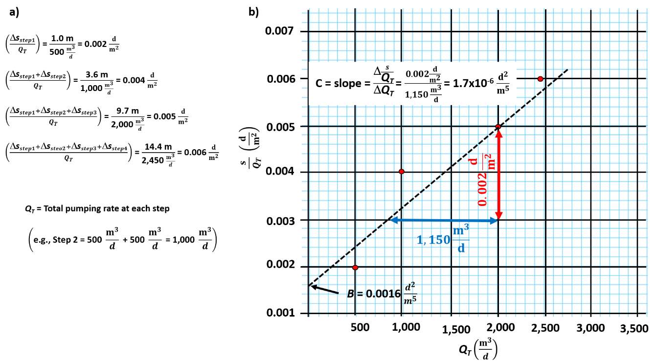
Figure 87 ‑ Example of a Hantush‑Biershenk plot used to analyze steady‑state step‑drawdown data to determine the turbulent well loss coefficient, C, and the value of B. a) Calculations of values of QT, s, and s/QT for each step. b) Plot of s/QT for each step versus the total pumping rate (QT) at the step. The slope of a fitted straight line (dashed line) is the value C and the intercept of the fitted line on the y‑axis is the value B.
The well‑loss coefficient is derived from the slope of the fitted line shown in Figure 87. Given the scatter of the data in this example, C values will vary depending on the location of the fitted line. The well loss, sWL, from turbulent conditions is then calculated at a specified discharge as CQ2. The turbulent well‑loss coefficient described by Jacob (1950) is assumed to be a constant. For example, if the well producing the data shown in Figure 87 was being pumped at 2,500 m3/d, the turbulent well loss would be (0.0000017 d2/m5) (2,500 m3/d)2 = 10.6 m.
The coefficient B of Equation (87) is related to the formational properties and represents some linear well loss as discussed in previous sections. It is derived from the y‑axis intercept of the fitted straight line. If other time‑drawdown data collected from an observation well during a constant discharge pumping test are available, an estimate of B1 of Equation (87) can be derived using standard curve‑matching methods because the observation well is not pumped so it is 100 percent efficient.
Without an independent method to estimate B1, the value B derived from step test analyses is assumed to represent an estimate of the formational drawdown, sF = BQ. In that case, aquifer properties will be underestimated because the drawdown used to estimate B contains some undefined well loss, and thus is greater than the drawdown for only formational conditions, B1. When steady‑state conditions occur, the Thiem Equation can be applied to estimate T for confined conditions (Equations (89), (90), (91), and (92)).
| [latex]s_{T} = \ \frac{Q}{2\pi T}\ln\left( \frac{r_{0}}{r_{w}} \right) + CQ^{2}[/latex] | (89) | |
|---|---|---|
| [latex]s_{F} = s_{T} - CQ^{2}[/latex] | (90) | |
| [latex]s_{F} = BQ = \ \frac{1}{2\pi T}\ln\left( \frac{r_{0}}{r_{w}} \right)Q[/latex] | (91) | |
| [latex]B = \ \frac{1}{2\pi T}\ln\left( \frac{r_{0}}{r_{w}} \right)[/latex] | (92) |
where:
| B | = | coefficient for a confined aquifer under steady‑state conditions (TL‑2) |
|---|---|---|
| T | = | transmissivity (Kb) (L2T‑1) |
| Q | = | constant pumping rate (L3T‑1) |
| sT | = | static water level minus the head in the pumping well (L) |
| sF | drawdown attributed to formational properties (L) | |
| rW | = | radius of the pumping well (L) |
| r0 | = | radial distance where drawdown equals 0 (estimated) (L) |
The pumping‑well radius is derived from the well‑construction information. However, when a gravel pack is present the well radius is often replaced by the effective well radius; that includes the screen radius and radius of the surrounding gravel pack. The effective radius is then used as rw in the Thiem and Theis single‑well pumping equations.
When steady‑state unconfined conditions are present, the total and formational drawdowns are usually approximated assuming the saturated thickness only changes a small amount during pumping. This allows application of the equations for confined aquifers, Equations (89) through (92).
In Equation (92), the value of B is derived from the plot shown in Figure 87. The radius of the well is obtained from field measurements and well construction records. Once the value of B is graphically determined, values of T and K=T/b can be computed using Equation (92). However, the solutions depend on an estimate of the radial distance from the pumping well where drawdown is zero, r0. An arbitrary value of 500 m is often assumed for steady‑state confined conditions because it is sufficiently large and using another sufficiently large value makes little difference in the result. When pumping rates are high, assumed distances can be increased by 1.5 to 2 times. Estimates of T change with different radial‑distance values (zero drawdown). However, because the radial distance is divided by the well radius and the natural logarithm is applied to the ratio, final estimates vary slightly when larger or smaller distances are used.
Results of a transient step‑drawdown test such as the one shown in Figure 86 can be analyzed using the same approach as described in Figure 87. Figure 88 is a plot of s/QT versus QT for the transient test. Values of s/QT for each step are computed using drawdown values measured at the end of the designated constant time, in this case the first 30 minutes.
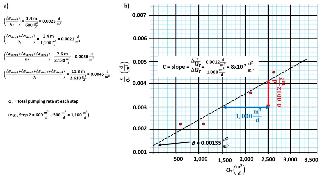
Figure 88 ‑ A Hantush‑Biershenk plot used to analyze transient step‑drawdown data to determine the turbulent well loss coefficient, C, and the value of B in a confined system. a) Calculations of values of QT, s and s/QT for each step using drawdown at the end of the 30‑minute interval since the step began. b) Plot of s/QT for each step versus the total pumping rate (QT) at the step. The slope of a fitted straight line (dashed line) is the value C and the intercept of the fitted line on the y‑axis is the value B.
Again, using the relationship shown in Equation (88) shows BQ = sF. Estimates of T will be higher if only B1 is used. Defining B using the Cooper‑Jacob approximation for a confined aquifer for u<0.01 yields Equation (93).
| [latex]B = \frac{1}{4\pi T}\ 2.30\ log\left( 2.25\ \frac{Tt}{r_{w}^{2}S} \right)[/latex] | (93) |
|---|
where:
| B | = | formational coefficient for transient conditions (TL‑2) |
|---|---|---|
| T | = | transmissivity (L2T‑1) |
| t | = | constant time step length corresponding to the reported drawdown value (T) |
| rW | = | radius of the pumping well (L) |
| S | = | storativity (dimensionless) |
Transient estimates of Β require an estimate of S. This is often derived by estimating the specific storage (Ss) of the aquifer material and computing a value of S =Ss (as discussed in Box 2). In addition, the estimate of B is time dependent. Thus, it is not used to estimate formational drawdown at other than early times (length of a step). The computed T values and estimates of S can be used to compute drawdowns at other times using appropriate analytical solutions (confined aquifer). If sufficient time‑drawdown data are collected in the first step of the step test these data can be corrected for non‑linear well loss and then used to curve match and compute additional estimates of T and S.
Jacob (1950) developed another method to estimate C using at least three consecutive steps from a step‑drawdown test. Most often this method is used for confined transient conditions and the change in drawdown is compared for equal time intervals since the step began, drawdown after 30 minutes or 1 hour for example (Figure 86). The turbulent well‑loss coefficients bracketed by two pumping rates are computed as shown in Equations (94), (95), and (96).
| [latex]C_{1} = \frac{\left( \frac{\mathrm{\Delta}s_{step2}}{\mathrm{\Delta}Q_{2}} \right) - \left( \frac{\mathrm{\Delta}s_{step1}}{\mathrm{\Delta}Q_{1}} \right)}{\mathrm{\Delta}Q_{1} + \mathrm{\Delta}Q_{2}}[/latex] | (94) | |
|---|---|---|
| [latex]C_{2} = \frac{\left( \frac{\mathrm{\Delta}s_{step3}}{\mathrm{\Delta}Q_{3}} \right) - \left( \frac{\mathrm{\Delta}s_{step2}}{\mathrm{\Delta}Q_{2}} \right)}{\mathrm{\Delta}Q_{2} + \mathrm{\Delta}Q_{3}}[/latex] | (95) | |
| [latex]C_{3} = \frac{\left( \frac{\mathrm{\Delta}s_{step4}}{\mathrm{\Delta}Q_{4}} \right) - \left( \frac{\mathrm{\Delta}s_{step3}}{\mathrm{\Delta}Q_{3}} \right)}{\mathrm{\Delta}Q_{3} + \mathrm{\Delta}Q_{4}}[/latex] | (96) |
where:
| C1, C2, C3 | = |
well loss turbulence coefficient for steps 1‑2, 2‑3 and 3‑4 (T2L‑5) |
|---|---|---|
| ∆sstep1, ∆sstep2, ∆sstep3, ∆sstep4 | = |
drawdown for each step after a constant pumping period (L) |
| ∆Q1, ∆Q2, ∆Q3, ∆Q4 | = | changes in pumping rates between steps (L3T‑1) |
C can be computed based on the response of two sequential steps using the transient step‑drawdown data shown in Figure 86. Some researchers discourage using this approach because in the original formulation of C it is assumed to be constant (Jacob, 1950). However, often when this method is used most C values show variability. When values of C are similar, they can be averaged or a value more representative of the pumping rate selected is used to compute well loss.
Example
Using Jacob’s method (1950) compute C from the transient data set shown in Figure 86, the time interval for analysis of each step is 30 minutes from the beginning of the step.
| [latex]C_{1} = \frac{\left( \frac{1\ m}{500\frac{m^{3}}{d}} \right) - \left( \frac{1.4\ m}{600\frac{m^{3}}{d}} \right)}{600\frac{m^{3}}{d} + 500\frac{m^{3}}{d}} = - 3.0x10^{- 7}\frac{m^{5}}{d^{2}}[/latex] |
|---|
| [latex]C_{2} = \frac{\left( \frac{5.2\ m}{1030\frac{m^{3}}{d}} \right) - \left( \frac{1.0\ m}{500\frac{m^{3}}{d}} \right)}{500\frac{m^{3}}{d} + 1030\frac{m^{3}}{d}} = 2.0x10^{- 6}\frac{m^{5}}{d^{2}}[/latex] |
| [latex]C_{2} = \frac{\left( \frac{4.2\ m}{480\frac{m^{3}}{d}} \right) - \left( \frac{5.2\ m}{1030\frac{m^{3}}{d}} \right)}{1030\frac{m^{3}}{d} + 480\frac{m^{3}}{d}} = 2.4x10^{- 6}\frac{m^{5}}{d^{2}}[/latex] |
The coefficients are used to compute the additional drawdown caused by non‑linear well loss. The negative value computed between the first two steps suggests the well was developing when pumped at 1,100 m3/d in the second step. If a step‑drawdown test is completed and then followed by a constant discharge pumping test using the single well, the computed well loss (additional drawdown) for that pumping rate would be subtracted from the observed drawdown data before time‑drawdown data were analyzed to estimate T and S.
Well Interference
It is best if other nearby wells are not operating during a single pumping test. However, if the operating schedules of surrounding wells in the area are known, well interference can be computed using standard analytical solutions or they can be observed during non‑pumping test periods. This involves monitoring water levels prior to and after pumping to see if adjacent pumping wells are impacting the water levels at the test well. If the effects of pumping in the surrounding wells are observed in the time‑drawdown data of the test well, they can be removed as described in Section 11.1. Observed drawdown may be affected during both drawdown and recovery.
Other Conditions that Effect Pumping Well Drawdown
Other factors may influence water levels during a single‑well test
- wellbore storage effects can occur, and are more pronounced for larger‑diameter wells and lower pumping rates;
- confined systems can be affected by barometric pressure changes, tidal loading, and direct loading; and
- unconfined systems may be impacted by tidal loading, evapotranspiration cycles, river‑stage changes, and short‑ or long‑term recharge events.
Wellbore‑storage effects were discussed in Section 12.1. Additional details on the effects of changing barometric pressure as well as both tidal and direct loading on observed water levels are discussed in Section 5. Water‑level changes in the pumping well due to these factors will be small in most cases. These factors will have a greater effect on late‑time data when drawdown changes due to formational conditions are also small. If time‑drawdown data need to be corrected for these perturbations, Kruseman and de Ridder (2000) and Sterrett (2007) provide a list of corrections. Procedures for determining production‑well efficiency are described in Box 4.