
12.2 Drawdown and Recovery Curve Matching Methods for a Single Pumping Well
Time‑drawdown and recovery data for a single pumping well can be analyzed using the appropriate analytical solutions and standard curve‑matching methods discussed in previous sections. Automated software analysis can also be applied (Section 13). Data need to be corrected for partial‑penetration and well‑loss effects before curve matching as described in Section 12.1.
Analyzing Time‑Drawdown Data
Drawdown corrections discussed in Section 5 and Sections 12.3 through 12.5 will produce drawdown data sets that represent formational aquifer properties. The Theis, Cooper‑Jacob, Hantush, Neuman, and other methods can be applied to estimate T and S. Log‑log data plots can be matched with type curves or by using numerical methods, and as appropriate, semi‑log plots analyzed to yield aquifer properties and properties of confining units (e.g., leaky confining units). Specific examples are not provided here because they are discussed in Sections 8 through 10.
If single‑well time‑drawdown data are not corrected for well loss or partial penetration, curve‑matching and straight‑line analytical methods will still provide reasonable estimates of T, but poor estimates of S. This is because the effects of well loss at a constant pumping rate and partial penetration are constant. These conditions increase the drawdown by fixed quantities. This results in maintaining the shape of data plotted on log‑log scales and the slope of data plotted on semi‑log scales. Thus, curve‑matching techniques result in match points with reasonable values of the well function and drawdown, and poor values for integration variables like u and time as illustrated in Figure 89.
This is an important conclusion. It means that a carefully conducted pumping test without observation wells may be well worth the cost. Together with the step drawdown tests such a pumping test can provide robust estimate of field‑scale transmissivity near the pumped well in addition to information on the efficiency of the well.
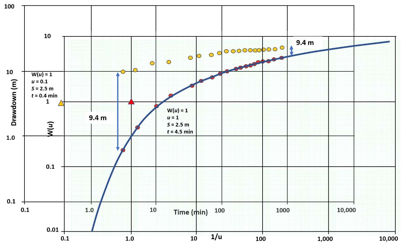
Figure 89 ‑ Time‑drawdown data for a pumping well completed in a confined water‑bearing unit. Orange solid dots represent field‑collected data at the pumping well and red solid dots show corrected drawdown at the pumping well if partial penetration and/or well loss is occurring. This example shows an offset (lower water levels) of 9.4 m. Curve matching methods conducted on both data sets yield match point values shown as orange (uncorrected, curve matching not shown) and red (corrected) triangles. W(u) and s are equal at both of the selected match points while u and t are different. Calculations of T from uncorrected time‑drawdown data (orange dots) yield good estimates of T (compared with the corrected computed T), but poor estimates of S. Once again, S can be approximated using methods presented in Box 2.
An example of another set of corrected and uncorrected single‑well drawdown data analyzed using the Cooper‑Jacob straight‑line method is shown in Figure 90. The slope of the lines is the same, so the calculation of T yields the same values for both curves. This is because the Cooper‑Jacob method does not rely on the absolute magnitude of the drawdown as the Theis method does. It depends on the rate of change of drawdown. However, the straight‑line intercept, t0, is smaller for the uncorrected field data set impacted by the 6 m offset (Figure 89). The storativity calculation is dependent on the magnitude of the drawdown. Analyzing uncorrected drawdown data will yield a poor estimate of S.
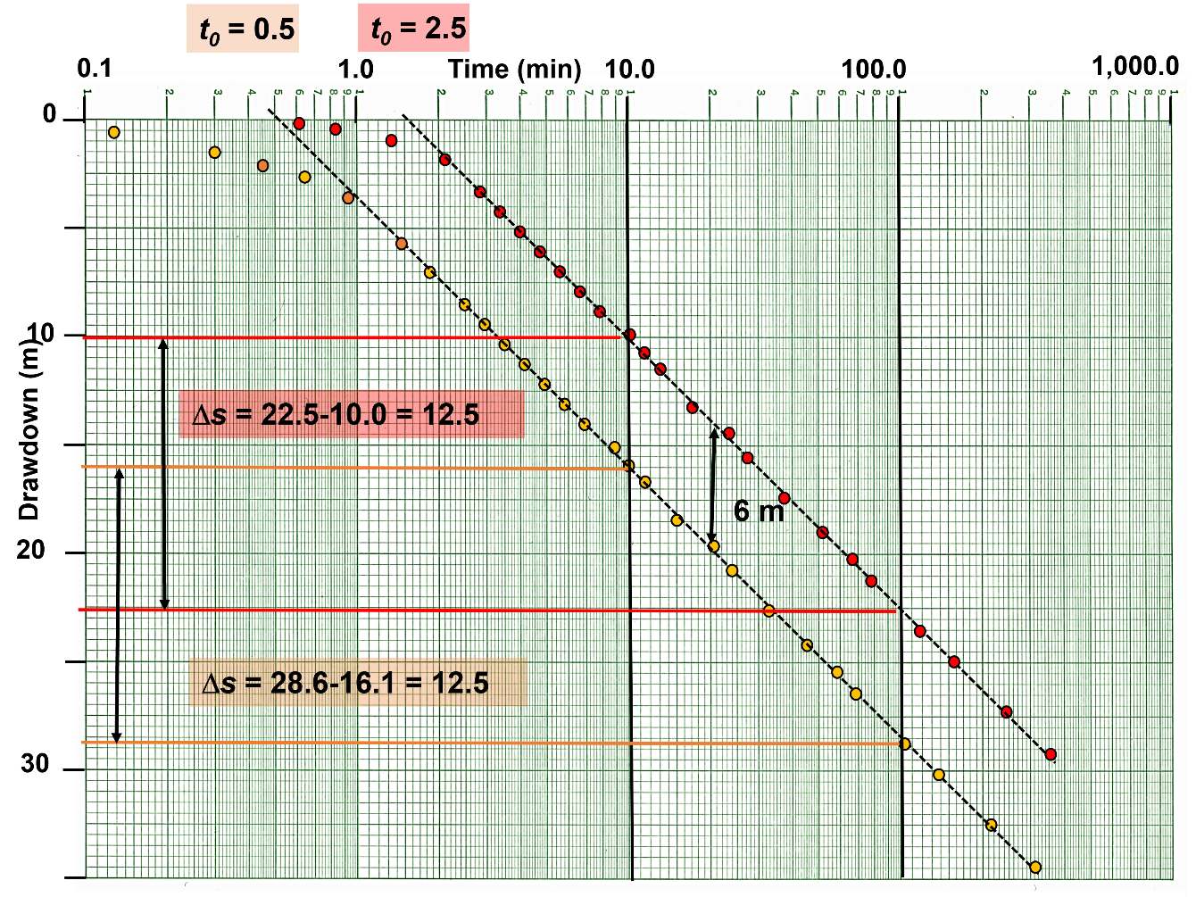
Figure 90 ‑ Time‑drawdown data for a pumping well finished in an isotropic and homogeneous confined aquifer. Orange solid dots represent field data collected at the pumping well and red solid dots show the formational drawdown at the pumping well if the effects of partial penetration and/or well loss are not occurring (corrected data). This example shows an offset (lower water levels) of 6 m. The slope of the two lines is the same. Calculations of T from uncorrected time‑drawdown data (orange dots) yield the same T value as that derived from the corrected data (red dots). Since the lines are offset by additional drawdown the t0 intercept used to calculate S is smaller for the field‑measured drawdown than the corrected data set. As a result, the uncorrected data set represented by the orange dots will yield a poor estimate of S. Once again, if only uncorrected drawdown data are available, S can be approximated using methods described in Box 2.
Analyzing Recovery Data
Plots of calculated‑recovery or residual‑recovery (Section 8, Figure 36) data collected after shutdown of a single‑well pumping test can be used to compute estimates of T and S. Partial‑penetration effects are present during recovery and require correction of recovery data before analysis as described above.
The effect of well loss on recovery data is different than on drawdown data. Once the pump is shut off, the well‑loss‑impacted water level in the borehole is lower than the head directly outside the casing as shown in Figure 91. This results in rapid flow of water into the well bore until water levels inside and outside the casing are equal. Once this occurs water‑level recovery is based on formational properties and no well‑loss correction is required (Figure 91).
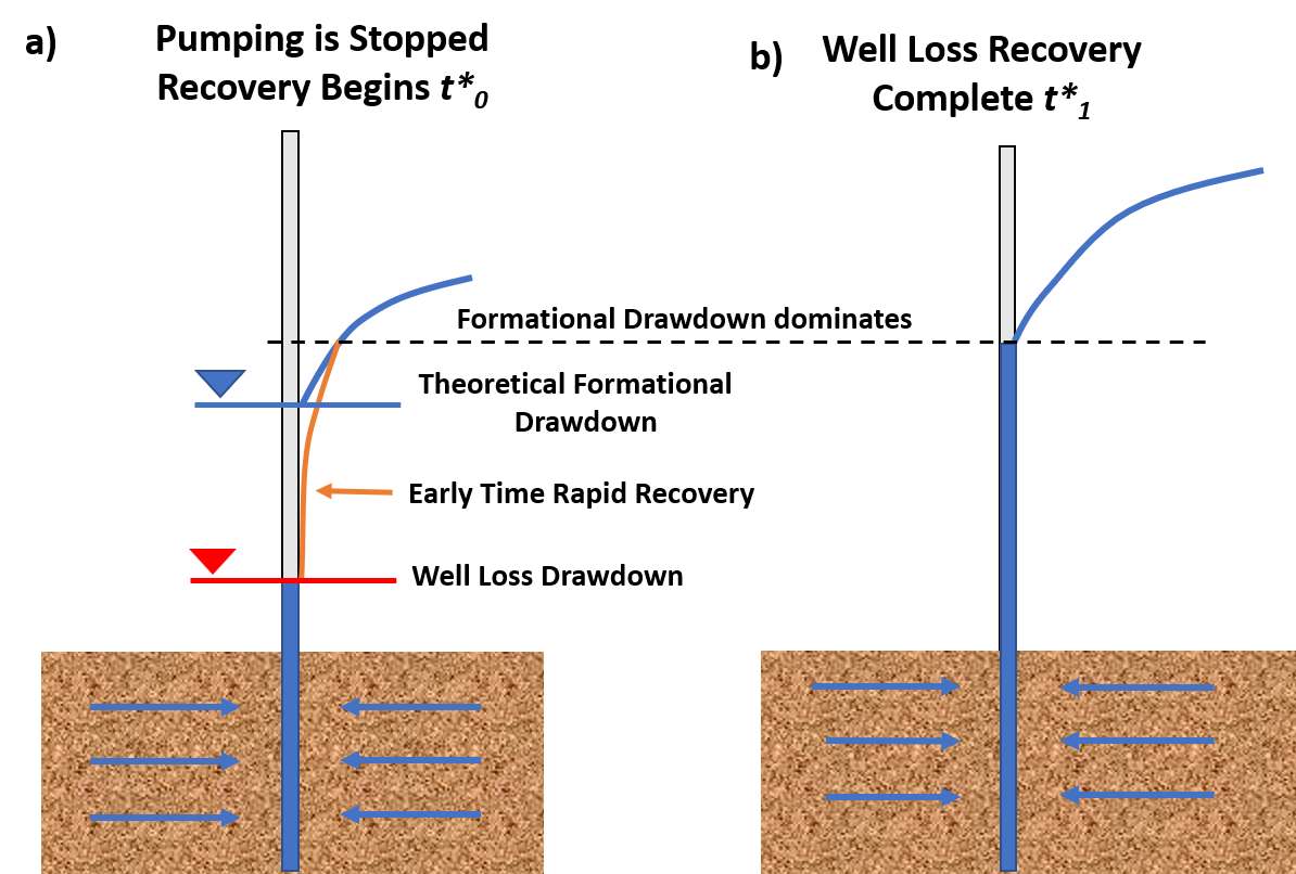
Figure 91 ‑ Schematic of the effect of well loss on the pumping level during recovery for an isotropic and homogeneous confined aquifer. The blue line represents the theoretical formational drawdown level at the end of pumping if well loss is not present. The red line represents the effect of well loss at the end of pumping. a) Well loss causes the water level in the pumping well to be lower than if the well loss was zero. The sketch shows the position of the water level (red) when the pumping is complete and the pump is shut off, t*0. The orange line represents the borehole water‑level response once recovery begins. After the pumping stops water continues to move to the well under the field gradients. The steep gradient near the well between the water level in the wellbore (well loss level) and the head immediately outside of the wellbore (formational head) results in rapid flow of water into the well bore and rapid recovery of the water level in the pumping well so that it soon reflects the formational water level at the well radius (often within minutes of shutting off the well). b) After this, water level recovery in the pumping well follows the formational response. This later time‑recovery data can be used to estimate T and S.
Hargis (1979) reported an example of the water level in a 40 percent efficient well that recovered to formational drawdown levels within four minutes after one day of pumping. Well‑loss effects are negated once this resetting of the recovery water level has occurred. By ignoring early‑time recovery data, the remaining water‑level data will produce representative aquifer properties if the well is fully penetrating, and no other influences are affecting recovery water levels. Examples of the effect of well loss on early recovery data are illustrated in Figure 92.
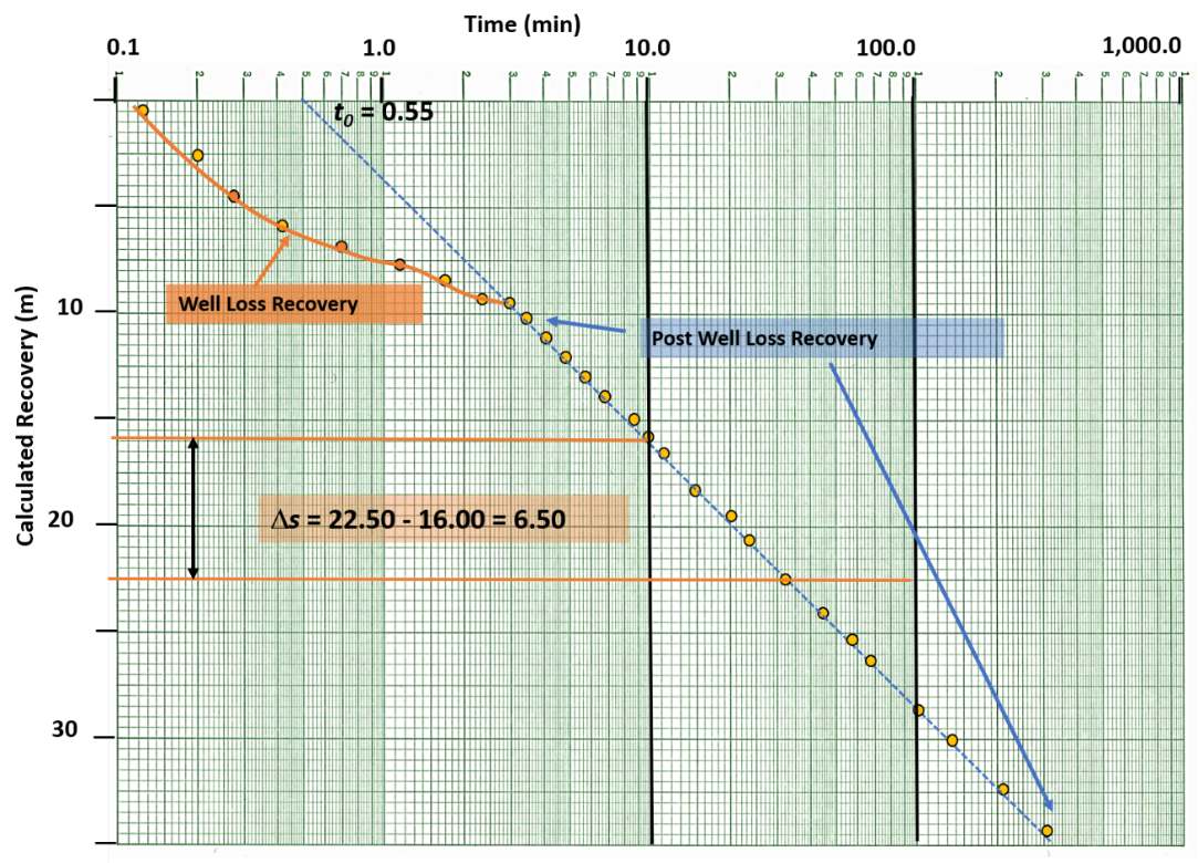
Figure 92 ‑ Schematic of a log‑log plot of calculated recovery data impacted by well loss for single‑well pumping in an isotropic and homogeneous confined aquifer. The early‑time data are impacted by the rapid rise in water levels caused by well loss recovery. The later time data, in this example after 10 minutes, are unaffected by the early‑time change in water levels caused by well‑loss recovery. A dashed blue line is fitted to the late‑time data. If other additional conditions are not impacting the calculated recovery data (e.g., partial penetration) the calculated recovery data requires no further correction to estimate T and S.
If the well is partially penetrating, either the recovery data will need to be corrected to compute T and S, or as described in the drawdown section, log‑log plots and semi‑log plots can be used to compute T; however, S will be poorly estimated.