
12.4 Performance Tests, Specific Capacity Data, and Estimating T
A performance test is typically conducted when a new production well is completed. Tests are primarily performed to estimate well yields and can also be used to estimate values of T.
The performance test involves measuring the starting water level, pumping a well at a constant rate for a period of time, and measuring the ending water level (at the time the pump is shut down). Transmissivity of the geologic material in which the well is completed is estimated by coupling this test with well‑construction data that identifies the perforated interval and the degree of screen penetration, and geologic well logs to classify the water‑bearing unit as confined or unconfined. Often performance‑test data are provided on existing driller’s logs. When such records are available, analysis costs are reduced because fieldwork is not required. Certainly, a hydrogeologist can conduct a performance test on an existing well using its pump or by installing a test pump in an unused well. However, if a hydrogeologist is going to pump a well it would be better to measure drawdown over time and then use single‑well pumping‑test analysis techniques to estimate properties as described in Section 12.2.
Cautions when Using Performance Test Results
Analysis of performance‑test data often relies on the information a drilling contractor reports after completing a well. Data are most useful when a pump is used to produce the well yield. When new wells are completed, testing is often performed when the drill rig is still on the site before installing a pump. In these settings, static water levels are measured, and then water is either bailed or air‑lifted from the well by setting the drill stem below the static water level and lifting the water out of the well with compressed air (Sterrett, 2007). The reported pumping rates are usually estimated. When a bailer is used discharge is determined by knowing the approximate volume of the bailer used and the number of bails per minute. If water is airlifted the discharge is estimated by periodically noting the time required to collect a known volume (e.g., a 5‑gallon or 20‑liter bucket) or measured with a flow meter on the outlet. Discharge may not be constant; thus, the reported value contains uncertainty. Further uncertainty is introduced because the final pumping water level is difficult to measure when these methods are used to extract water. Once bailing is stopped some recovery may occur in the pumping well before the water level is measured. Some recovery may also occur after airlifting is completed. Unfortunately, often the depth of the suspended drill rod (airlifting) and not the actual measured water level is reported as the final pumping level. When a pump is set and used to conduct the test, pumping rates and water levels are usually more reliable. Performance‑test records should be used with caution and the realization that there is uncertainty in the reported flow rate and water levels. Professional judgment is needed to interpret the reported data.
The performance‑test drawdown cannot be corrected for well loss because a step‑drawdown test is not performed. If a step‑drawdown test was performed it should be used to estimate aquifer properties instead of the performance test and the component of drawdown attributed to well loss would be defined as discussed in Section 12.1. Depending on the well construction, partial penetration may also impact reported drawdowns. The pumping level would need to be corrected (Equation (80)). If drawdown data are not corrected for well loss and/or partial penetration, drawdowns will be greater than drawdown in a fully penetrating and 100 percent efficient well. As a result, computed values of T will be underestimated and should be considered to provide only an order‑of‑magnitude estimate.
Storativity is not computed from performance‑test data sets. Rather, it is estimated by the groundwater professional when transient conditions are assumed (Box 2). The selected value of S will result in only small changes to the estimated values of T.
Methods to Estimate Transmissivity from Performance Tests
First, it must be determined whether the well is completed in a confined or unconfined unit by assessing the reported geological sequence of materials, the static water level in the well, the driller’s reported first encounter of water (water table), and the location and extent of the perforated interval. Not all drillers’ logs have complete information on the first water encountered, so professional judgment, the geological literature, and nearby well logs are often required to assign the well to a confined or unconfined aquifer.
Using performance test data, T can be estimated by calculating the specific capacity of a well. Specific capacity is the well yield divided by the drawdown reported for the length of pumping time as in Equation (99). Generally, if multiple performance tests are examined and pumping durations are similar, the larger the specific capacity of a well the greater the T of the formation.
| [latex]Specific\ Capacity = \ \frac{Q}{s_{F}}[/latex] | (99) |
|---|
where:
| Q | = | constant pumping rate (L3T‑1) |
|---|---|---|
| sF | = | drawdown corrected for partial penetration and well loss at some time (L) |
However, specific capacity varies with time, becoming smaller as time and drawdown increase (Figure 95). Ideally, a representative specific capacity would only be reported once steady‑state conditions had been reached. However, this is rarely the case, as performance tests often only last one‑half hour to two hours. Methods used to estimate T from specific‑capacity data include interpreting data as representing steady‑state and transient conditions as discussed in Sections 12.4.3 through 12.4.5. However, aquifer‑property estimates computed using specific‑capacity data should be considered as reconnaissance level, rough estimates, or order of magnitude values. In many cases well and testing data may be incomplete, or several assumptions are required to apply equations making results more uncertain. However, when used with an appreciation for their limitations, methods to characterize aquifer properties can be useful.
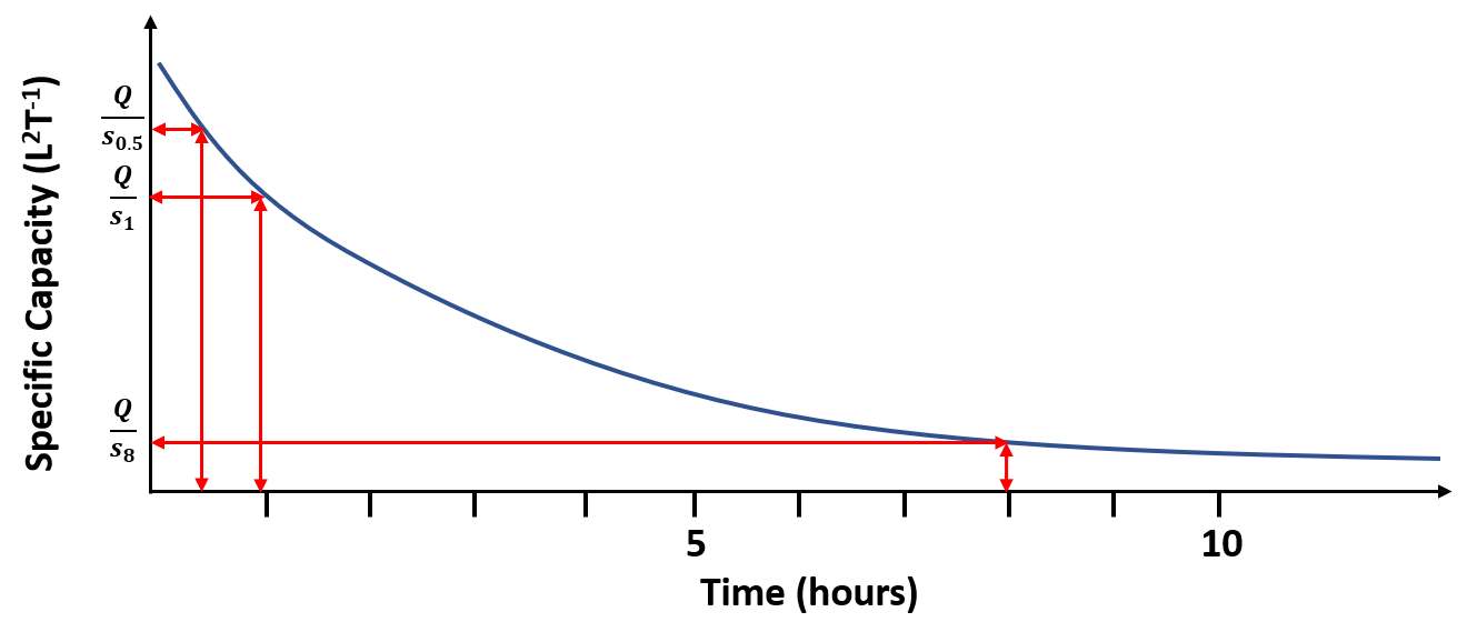
Figure 95 ‑ Schematic arithmetic plot of the transient change in specific capacity during pumping at a constant rate. The shape of the curve illustrates that head response to pumping is logarithmic. Computed specific capacities are higher at early times and smaller at later times. Q/s0.5 corresponds to the specific capacity computed after 0.5 h of pumping. In this illustration, the time scale suggests that changes in drawdown become small after 5 to 10 hours of pumping and thus changes in the computed values of specific capacity are also small. If drawdown reaches a steady state, the specific capacity becomes constant.
Using Specific Capacity to Estimate Transmissivity Assuming Steady‑State Conditions
As discussed in Section 12.3, when performance‑test data are assumed to represent drawdown at steady state, the corrected well drawdown (for partial penetration) can be used in the Thiem Equations (Equations (97) and (98)). For confined systems T is a function of the head at the pumping well (assigned to rw, the radius of the pumping well) and the head at the radial distance at which drawdown is zero, r0. Values of r0 are assumed to be 250 m and 500 m for unconfined or confined systems respectively. Again, as a caution, performance tests may not represent steady‑state conditions because pumping durations are often too short. Near steady‑state conditions can occur when pumping rates are low and water‑bearing materials are highly transmissive, and/or when recharge boundaries are encountered after short pumping times.
Using Specific Capacity Data to Estimate Transmissivity Assuming Transient Conditions
Well‑performance data can be used to estimate T when pumping duration is short and conditions are assumed to be transient. For example, if the test is run for only 30 min to an hour, it is likely that the recorded drawdown does not represent steady‑state conditions. Assuming the confined Cooper‑Jacob approximation can be used to represent transient conditions where S is estimated (for confined or unconfined conditions, Box 2) and the time used in the analyses is the duration of pumping recorded for the test, then the Theis assumptions are applied as shown in Equations (100) and (101).
| [latex]\frac{s}{Q} = \frac{1}{4\pi T}\ 2.30\ log\left( 2.25\ \frac{Tt}{r_{w}^{2}S} \right)[/latex] | (100) |
|---|
| [latex]\frac{Q}{s} = \frac{1}{\frac{1}{4\pi T}\ 2.30\ log\left( 2.25\ \frac{Tt}{r_{w}^{2}S} \right)}[/latex] | (101) |
|---|
where:
| s | = | corrected final drawdown (L) |
|---|---|---|
| Q | = | constant well discharge (L3T‑1) |
| T | = | transmissivity (L2T‑1) |
| log | = | logarithm base 10 |
| t | = | duration of the performance test (T) |
| rw | = | radius of the pumping well (L) |
| S | = | storativity (estimated) (dimensionless) |
The well radius is represented by the effective radius (screen radius + gravel pack radius) when a gravel pack is present.
A log‑log graphical solution to Equation (101) is obtained by plotting the Q/s versus T with values of T = 100, 1,000, and 10,000 m2/d substituted into Equation (101) along with the radius of the pumping well, the pumping rate, the length of time the well was pumped, and an estimate of S as discussed in Box 2 as shown in Figure 96.
Example
If a 0.15‑m‑radius well penetrating a confined aquifer with S = 0.0001 (estimated) is pumped for 30 minutes (0.02 d) and has a specific capacity of 4,000 m3/d / 9 m = 444.4 m2/d, then the corresponding Q/s for the values of T = 100, 1,000 and 10,000 m2/d are 86 m2/d, 743 m2/d, and 6,538 m2/d. A log‑log plot of the relationship is produced, and a straight line is fitted to the data. Then the specific capacity value derived from the performance test, 444.4 m2/d is used to determine the corresponding value of T, 600 m2/d as shown in Figure 96.
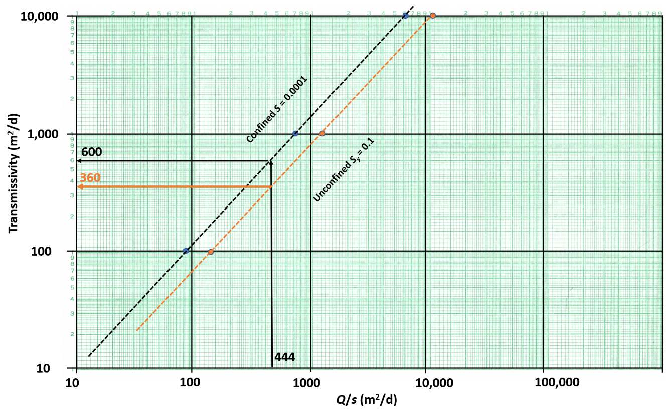
Figure 96 ‑ Log‑log plot of specific capacity and transmissivity for a 0.15 m radius well pumping at 4,000 m3/d for 30 minutes, and fully penetrating a confined aquifer with a storativity of 0.0001 (blue dots and black dashed fitted line). The specific capacity of the pumping well after 30 min (0.02 d) of pumping was 444 m2/d. The corresponding T value for a confined water‑bearing unit with the stated properties is 600 m2/d. If the penetrated material was unconfined with a storativity of 0.1, the values would be the orange dots which are fitted with the orange dashed line, and the result is shown with solid orange arrows. The corresponding transmissivity value is 360 m2/d.
The Cooper‑Jacob approximation can also be used to describe the general behavior of an unconfined unit without much change in saturated thickness near the pumping well.
Walton (1970) evaluated the positions and slopes of plots like those shown in Figure 96. He showed that at longer pumping times (>8 hours) fitted lines for the confined aquifer and unconfined aquifer changed little in position and had a constant slope. Todd and Mays (2005) show transient results of changes in specific capacity, storativity, and transmissivity for confined aquifers after 1 day of pumping at a constant rate (Figure 97).
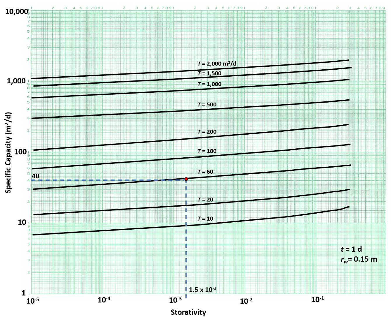
Figure 97 ‑ Relationship of specific capacity, storativity, and transmissivity for a single, 100 percent efficient, pumping well that fully penetrates a confined aquifer. The well has a radius of 0.15 m and is pumped for 1 day. T values are derived by selecting the specific capacity value and the storativity value (dashed blue lines) and then interpreting the value of T. In this example, the tested well has a specific capacity of 40 m2/d and a storativity of 1.5 X 10‑3, thus the estimated T value is 60 m2/d (modified from Todd & Mays, 2005; Bentall, 1963).
The transmissivity relationship for a fully penetrating, 100‑percent efficient well shown in Figure 97 is not very sensitive to the value of storativity (i.e., the lines are almost horizontal. The use of such plots assumes that Q/s is near steady state (declining very slowly) which may be a reasonable assumption after 1 full day of pumping a well at a constant rate. However, such long‑term pumping rates are rarely used when well performance tests are conducted (e.g., they are typically 30 minutes to 2 hours).
Basic Equations Relating Specific Capacity to Transmissivity
Kasenow (2001) thoroughly discusses how specific‑capacity data can be used to estimate transmissivity. Other authors have suggested simplified relationships between specific capacity and transmissivity like the graphical data presented in Figure 97. Driscoll (1986) and others suggested a general estimate of T from the specific capacity for a pumping well that penetrates a confined or unconfined aquifer could be obtained using Equations (102) and (103). These equations assume general properties of the formations. The duration of pumping is not considered, yet Q/s changes with time. These equations should be used cautiously as they assume Q/s is a representative value of groundwater conditions.
Transmissivity for confined conditions is estimated using Equation (102) as presented by Driscoll (1986).
| [latex]T = 1.39\left( \frac{Q}{s} \right)[/latex] | (102) |
|---|
Transmissivity for unconfined conditions is estimated using Equation (103) Driscoll (1986).
| [latex]T = 1.04\left( \frac{Q}{s} \right)[/latex] | (103) |
|---|
where:
| T | = | transmissivity (L2T‑1) |
|---|---|---|
| Q | = | constant discharge (L3T‑1) |
| s | = | drawdown in a fully penetrating and 100 percent efficient well (L) |
Studies of areas with both performance tests and pumping tests with observation wells have been used to develop empirical relationships between specific capacity and T. Razack and Huntley (1991) looked at over 200 pairs of performance and pumping tests for wells in an alluvial basin. They found that pumping test‑derived T values were underestimated by the specific‑capacity data. These differences were attributed to the presence of turbulent well loss in the specific‑capacity data. They generated the relationship for T shown in Equation (104).
| [latex]T = 15.3\ (Q/s)^{0.67}[/latex] | (104) |
|---|
where (in units of meters and days):
| T | = | transmissivity in m2d‑1 |
|---|---|---|
| Q | = | constant discharge in m3d‑1 |
| s | = | drawdown in a fully penetrating and 100 percent efficient well in m |
Using equations developed for specific study areas may not be appropriate as conditions for a particular well and hydrogeologic setting may be different than those from which a relationship was derived.
This section introduced several methods to estimate T using pumping and drawdown data from a single well. When possible, drawdown should be corrected for factors impacting the total drawdown such as partial penetration, well loss, well interference, and other factors described in this section. Well loss is best addressed by conducting a step‑drawdown test. However, when only performance‑test results are available, T can still be estimated, but the computed value is likely to be lower than the field value.
The best approach to using single‑pumping‑well data is to perform constant‑rate discharge tests where drawdown is measured over time. Analyses of such data allow the use of traditional curve‑matching and semi‑log plotting methods which produce more representative values of T.
The following section addresses how software tools are used to generate estimates of T and S. In most cases such programs apply analytical models with methods similar to curve matching to generate aquifer properties.