
14.4 Methods to Interpret Overdamped Slug Tests
This section presents the development, basic assumptions, and applications of the most common methods used to analyze overdamped slug‑test data. These methods include those developed by Hvorslev (1951), Bouwer and Rice (1976), Bouwer (1989), Cooper and others (1967), and Hyder and others (1994).
Hvorslev Slug Test Method
Hvorslev (1951) prepared a report for the Waterways Experiment Station Corps of Engineers, U.S. Army that addressed his experiments and observations examining how water levels in boreholes, piezometers, and monitoring wells responded when borehole water levels were purposefully raised or lowered. The report describes how formational hydraulic properties and the well design (shape factors) influence the water level recovery as a function of time.
Hvorslev (1951) developed a semi‑analytical solution applying a quasi‑steady‑state approach that assumes elastic storage can be neglected. Other simplifying assumptions include the formation being tested is isotropic, homogeneous, and uniform in thickness. The solution can be applied to partially or fully penetrating wells. The formulation is based on confined conditions. Analyses are applied to unconfined and confined systems. Falling‑head or rising‑head test data are analyzed using a semi‑log plot and an interpolated straight line (Figure 109).
Hvorslev (1951) developed several empirical equations to represent well designs in formations. There is no consideration of the water table as a fixed or moving boundary. His method allows for screens of varying diameters and lengths. In some settings well bores are only open at the bottom or can be partially filled with sediment. Notation used by Hvorslev (1951) is shown in Figure 111.
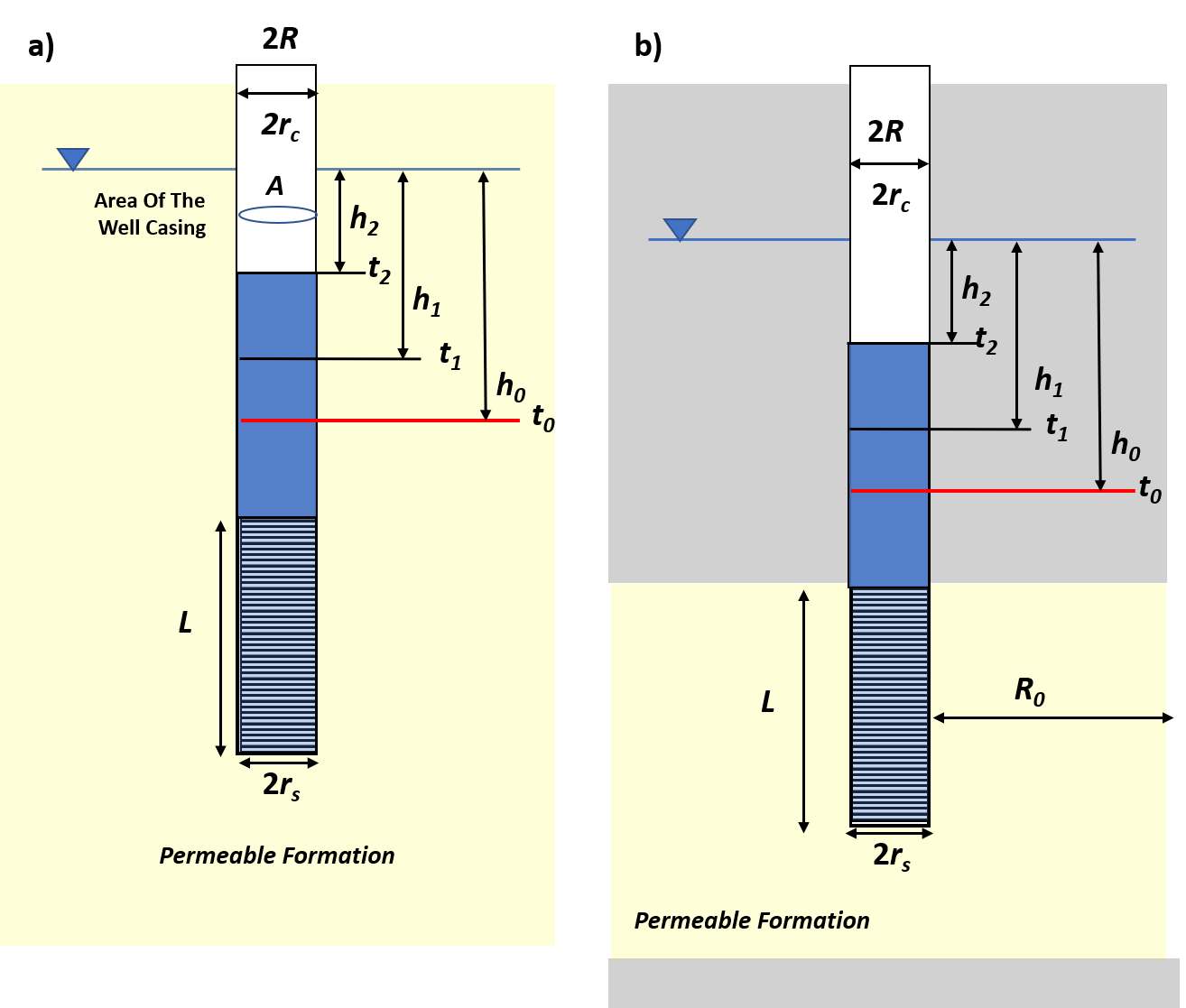
Figure 111 ‑ General notation for parameters used in the Hvorslev slug test method as defined for Equations (105) and (106). a) An example of a well completed in an unconfined system. b) An example of a well completed in a confined system (gray units are impermeable). R0 is the distance to the location where h does not change.
General equations describing the relationship between hydraulic conductivity, cross sectional area of the well, a shape factor representing the well configuration, and the slope of the of the normalized head, 1/(t2‑t1) ln (h1/h2), were formulated. Equation (105) shows the hydraulic conductivity is directly proportional to the area of the well casing and the slope of the slug test data, and inversely proportional to the well shape factor. The slope of the data plot is determined using the difference in two values of the normalized head at different times (h1 and h2) and difference in the two corresponding times (t1 and t2) (Figure 112). Hvorslev defines the normalized head Ht/H0 as H in his work. Equation (106) uses what is referred to as the basic time‑lag method to determine the slope of the slug‑test data. This approach represents the slope using the relationship that when the value of the normalized head equals 0.37 (log of 0.368 = ‑1) the corresponding time value can be read from the graph, T0.37 (Figure 112).
| [latex]K = \frac{A}{F}\left( \frac{1}{t_{2} - t_{1}} \right)\ln\frac{h_{1}}{h_{2}}[/latex] | (105) | |
|---|---|---|
| [latex]K = \ \frac{A}{F}\frac{1}{T_{0.37}}[/latex] | (106) |
where:
| Κ | = | hydraulic conductivity (LT‑1) |
|---|---|---|
| Α | = | cross‑sectional area of the well casing, πrc2 (L2) |
| F | = | shape factor that for some configurations is dependent on one or more of L, R, rc, rs (dimensionless) |
| h1 | = | normalized head at time t1 (L) |
| h2 | = | normalized head at time t2 (L) |
| t1 | = | time at head h1 (T) |
| t2 | = | time at head h2 (T) |
| T0.37 | = | basic time lag (T) |
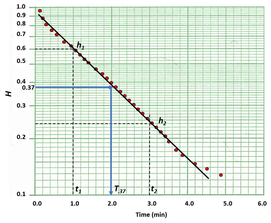
Figure 112 ‑ Semi‑log plot of slug test results (red dots) and a fitted straight line. The slope of the line is determined by two points of normalized head values (H), h1 and h2 and time values t1 and t2. The normalized head on the graph (H) is the unrecovered head measured from the static water level divided by the depth or height to which the water level drops or rises at the beginning of the test (measured from the static water level), which is Ht/H0 as shown in Figure 111. Also shown is the procedure for reading T..37 from the graph for use in the time lag method where the Ht/H0 value is 0.37.
The shape factor in Equations (105) and (106) is empirically derived for the well configuration and position in the formation being tested using analytical solutions for steady‑state flow. General well notations are presented in Figure 111. Four shape factors and equations to compute K for unconfined settings and two sets of conditions for confined settings are included in Figure 113. Figure 114 provides graphs of empirical constants and an equation for determining K in an unconfined anisotropic setting.
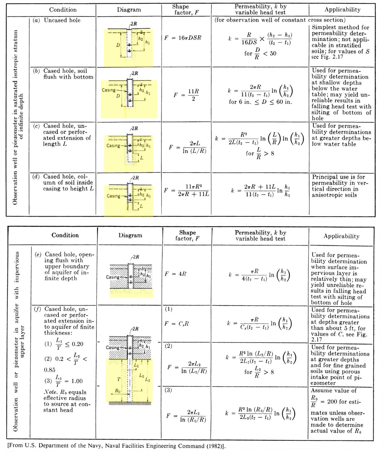
Figure 113 ‑ Well conditions, shape factors, and equations to compute hydraulic conductivity (K = permeability, k, on the table). Figure 114 is the figure referred to as 2.17 in the text in the left‑hand column. Values of Cs and S are also defined on Figure 114 (US Department of the Navy, 1982).
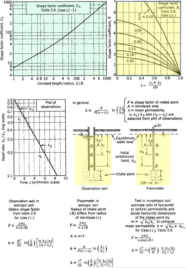
Figure 114 ‑ The empirical constant, Cs in relation to L/R (US Department of the Navy, 1982). This is the figure referred to as 2.17 in the text of Figure 113. The shape factor chart for S in the upper right‑hand corner is modified from Spangler (1963). Permeability is equivalent to hydraulic conductivity. F is the shape factor. Other parameters are defined in the text and in Figure 111 and Figure 113. The lower right hand corner diagram and text present a shape factor for an anisotropic formation in an unconfined setting.
Hydrogeology textbooks often include only a single equation for the Hvorslev method that is identical to condition (c) in Figure 113 and the equations in the lower left‑hand portion of Figure 114. The equation has the criteria that the ratio of L/R > 8 which is the case in most small‑diameter monitoring wells or piezometers where the screen length (L) is much greater than the radius of the casing (R). The equation includes the shape factor shown in Figure 113c. Condition (c) of Figure 113 is associated with Equations (107) and (108). These equations account for a difference in the well casing (rc) and screen radius (rs). The screen length is defined as the effective screen length and the screen radius also includes the gravel pack if present as shown in Figure 115b. Either Equation (107) or (108) can be used to compute K (Figure 113c). Figure 115 is a schematic of the properties used to develop Equations (107) and (108).
| [latex]K = \frac{{r_{c}}^{2}\ln\left( \frac{L_{e}}{r_{s}} \right)}{2\ L_{e}\ \left( t_{2} - t_{1} \right)}\ln\left( \frac{h_{1}}{h_{2}} \right)[/latex] | (107) | |
|---|---|---|
| [latex]K = \frac{{r_{c}}^{2}\ln\left( \frac{L_{e}}{r_{s}} \right)}{2\ L_{e}\ T_{0.37}}[/latex] | (108) |
where:
| h1/h2 | = | ratio of values used to define the slope (dimensionless) |
|---|---|---|
| t2‑t1 | = | times corresponding to the change in the normalized head, h2 and h1 (T) |
| Le | = | effective length of well screen (L) |
| rc | = | radius of the casing (L) |
| rs | = | radius of the screen interval (L) |
| T0.37 | = | time associated with the value of Ht/H0 = 0.368 (T) |
| K | = | hydraulic conductivity (LT‑1) |
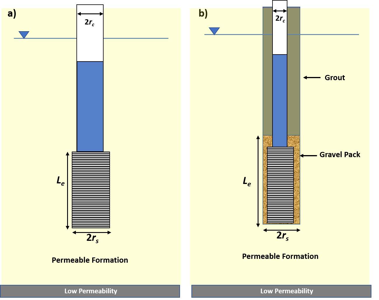
Figure 115 ‑ The parameters used to solve for the hydraulic conductivity as defined in Equations (107) and (108). Le is the effective length of the well screen. a) A well design where the radius of the well screen is larger than the radius of the well casing. b) A gravel packed well where the effective well screen radius and effective length of the well screen include well screen and gravel pack.
The effective well screen length, Le is the length of screen or the length of the gravel pack surrounding the screen. The screen radius also includes the gravel pack dimensions when present. In some shape functions (e.g., the f(3) of Figure 113) a value referred to as the effective radius of the slug test (Ro) is specified. This represents the distance the casing water flows from a falling‑head test into the formation or the distance formational water travels to the well in a rising‑head test. The value is empirical and generally assumed to be either the length of the well screen (Le) or 200 times the effective radius of the well screen (including the gravel pack when present) (US Department of Navy, 1982; Butler, 1996). Re is used as the effective radius of influence in other slug‑test methods (e.g., Bouwer & Rice, 1976).
Example
Assume a slug test was completed in a screened well penetrating an unconfined formation designed as shown in Figure 116.
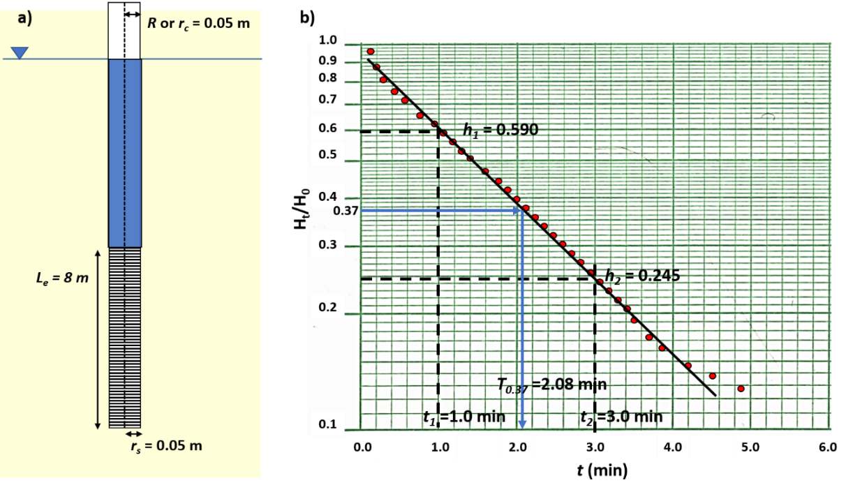
Figure 116 ‑ Well design and slug‑test data collected during the testing of an unpumped well. a) Well parameters. b) Semi‑log plot of slug‑test results. Values of h1, t1, h2, t2 and the time lag T0.37 are shown.
Examining the well design and recognizing it is constructed in an unconfined aquifer the method presented in Figure 113c is appropriate if the constraint that Le/R>8 is met; that factor is checked, 8 m / 0.05 m = 160, so the criteria is met. Thus, Equation (107) is applied.
[latex]K = \frac{{r_{c}}^{2}\ln\left( \frac{L_{e}}{r_{s}} \right)}{2\ L_{e}\ \left( t_{2} - t_{1} \right)}\ln\left( \frac{h_{1}}{h_{2}} \right)[/latex]
[latex]K = \frac{{(0.05\ m)}^{2}\ln\left( \frac{8\ m}{0.05\ m} \right)}{2\ (8\ m)\ (3\ minutes\ - \ 1\ minute)}\ln\left( \frac{0.59\ m}{0.245\ m} \right) = 0.00035\frac{m}{minute}[/latex]
[latex]K = 0.0003\frac{m}{minute}\frac{1440\ minute}{1\ day} = 0.50\frac{m}{day}[/latex]
The hydraulic conductivity can also be computed using the time‑lag equation, Equation (108).
[latex]K = \frac{{r_{c}}^{2}\ln\left( \frac{L_{e}}{r_{s}} \right)}{2\ L_{e}\ T_{0.37}} = \frac{{(0.05\ m)}^{2}\ln\left( \frac{8\ m}{0.05\ m} \right)}{2\ (8\ m)\ (2.08\ minutes)} = {0.00038}\left( \frac{m}{minute} \right)[/latex]
[latex]K = 0.00038\frac{m}{minute}\frac{1440\ minute}{1\ day} = 0.54\frac{m}{day}[/latex]
Though the values are not identical, this is expected as readings of parameter values from the graph will contain some degree of error.
Bouwer and Rice Slug‑Test Method
The Bouwer and Rice method is based on the work of Bouwer and Rice (1976) and Bouwer (1989). The underlying conceptual model is identical to the Hvorslev analysis. The Bouwer and Rice method uses a different representation for the shape factor.
The test methodology is applicable to open boreholes and wells fully or partially penetrating unconfined formations. The water table is a fixed boundary rather than a boundary that may be affected by testing. It can be used in confined conditions if the upper confining unit is leaky with an aquiclude as the lower boundary. Formations are assumed to be of constant thickness and infinite in lateral extent; the water table is near horizontal and does not change during the test, and formation‑storage effects are negligible. It is assumed conditions are isotropic and homogeneous and the saturated thickness of the formation being tested does not change. Also, water‑level changes induced by slug testing are assumed to be instantaneous (Kruseman & de Ritter, 2000).
The method is based on a mathematical model founded on the steady‑state governing equation for radial flow. The parameter definitions are shown in Figure 117. Field data are plotted as the log of the remaining drawdown with time (Figure 118).
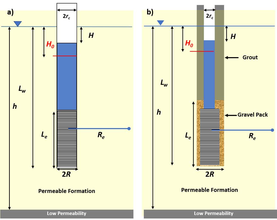
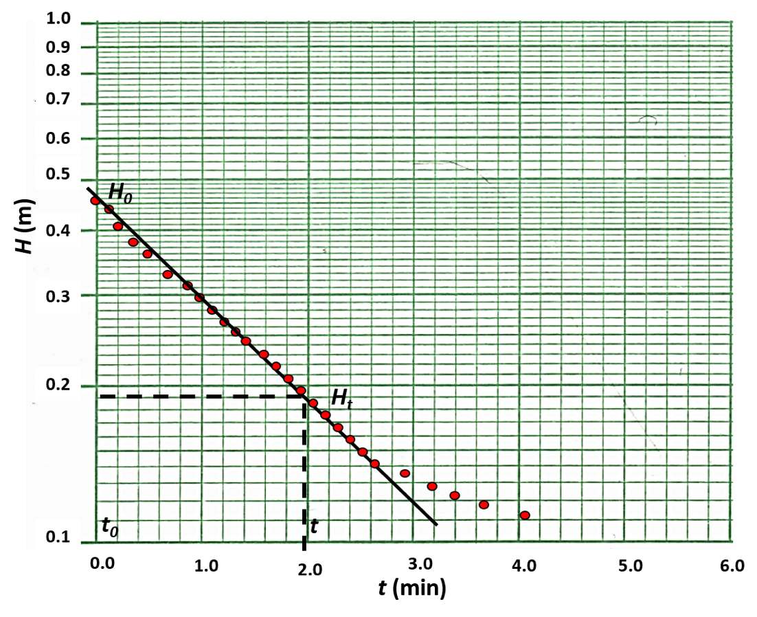
Figure 117 ‑ Definitions of parameters used in the Bouwer and Rice method. This example shows the response to a rising head test where H0 is the drawdown at t0 and H is the remaining drawdown at time t. Re is the effective radius of the slug test. a) A well where the radius of the well casing and well screen are the same. b) A setting where the well casing radius is smaller than the well screen radius. The screen length, Le, includes the gravel‑pack length. The screen radius, R, also includes the radius of the gravel pack when present.
Figure 118 ‑ Semi‑log data plot of a rising head slug test. The log of the value H (remaining drawdown) is plotted over time. The initial value of H is H0.
A straight‑line is fitted to the early time data (Figure 118). Issues discussed in the section on overdamped responses should be considered (Figure 109) when fitting a straight line to the semi‑log plots.
Bouwer and Rice (1976) developed an analytical solution with several empirical parameters as shown in Equation (109) (Butler, 1998). Parameters are illustrated in Figure 117.
| [latex]K = \frac{{r_{c}}^{2}\ln\left( \frac{R_{e}}{R} \right)}{2\ L_{e}t}\ln\frac{H_{0}}{H_{t}}[/latex] | (109) |
|---|
where:
| H0 | = | maximum water level change (drawdown in a rising head test at time t0) (L) |
|---|---|---|
| H or Ht | = | remaining drawdown in a rising head test at time t (L) |
| t | = | the time associated with Ht (T) |
| rc | = | radius of the casing (L) |
| R | = | radius of the screened interval including the gravel pack if present (L) |
| Le | = | effective length of the screen including the gravel pack if appropriate (L) |
| Re | = | the effective radius of the slug test influence (L) |
| K | = | hydraulic conductivity (LT‑1) |
The parameter Re represents the radius of influence of the slug test in the formation. This is defined as an empirical value. It is computed as a constant, ln(Re/R). Bouwer and Rice (1976) and Bouwer (1989) estimate the dimensionless ratio of ln(Re/R) in Equation (109). Considering Figure 117, they used two approaches for this estimate based on the position of the well in the unconfined formation. The estimation process includes additional non‑linear empirical constants that are derived from Figure 119 or computed from the equations defining the curves which are provided by (Butler, 1998, p. 109).
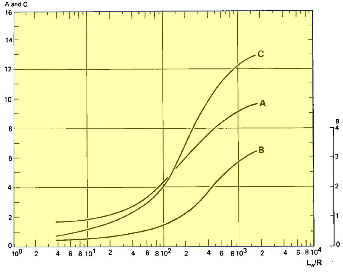
Figure 119 ‑ Empirical constants used in the Bouwer and Rice method estimate of ln (Re/R) (Kruseman & de Ritter, 2000).
If conditions are such that Lw, the distance of the bottom of the well from the water table, is less than h, the saturated thickness of the aquifer (Figure 117), then Equation (111) is applied to estimate ln(Re/R). Parameters for Equation (110) and Equation (111) are defined in Figure 117. Empirical parameters A, B and C are derived from Figure 119. If Lw equals h, then Equation (111) is used.
| [latex]\ln\left( \frac{R_{e}}{R} \right) = \left( \frac{1.1}{\ln\left( \frac{L_{w}}{R} \right)} + \left( \frac{(A + B)\ ln\left\lbrack \frac{h - L_{w}}{R} \right\rbrack}{\frac{L_{e}}{R}} \right) \right)^{- 1}[/latex] | (110) | |
|---|---|---|
| [latex]\ln\left( \frac{R_{e}}{R} \right){= \left\lbrack \frac{1.1}{\ln\left( \frac{L_{w}}{R} \right)} \right.\ + \left. \ \frac{C}{\frac{L_{e}}{R}} \right\rbrack}^{- 1}[/latex] | (111) |
Zlotnik (1994) developed a method to account for anisotropic conditions in the formation being slug tested. He defined R, the radius of the well screen, as R* = R(Kz/Kr)0.5, where Kz is the vertical hydraulic conductivity and Kr is the radial or horizontal hydraulic conductivity. The value R* is substituted for R in Equations (109) through (111) when conditions are anisotropic. Slug testing does not provide direct measurement of the vertical hydraulic conductivity. Estimates of vertical hydraulic conductivity are often assumed to be an order of magnitude smaller than horizontal values in stratified rock or sediments. However, in some settings horizontal to vertical hydraulic conductivity ratios can be 1000:1 (Anderson et al., 2015).
Example
If the data plotted in Figure 118 represent a rising‑head slug test (slug out of a well), and the formation tested is isotropic, homogenous, and unconfined as shown in Figure 120, then the hydraulic conductivity can be computed using Equation (109).
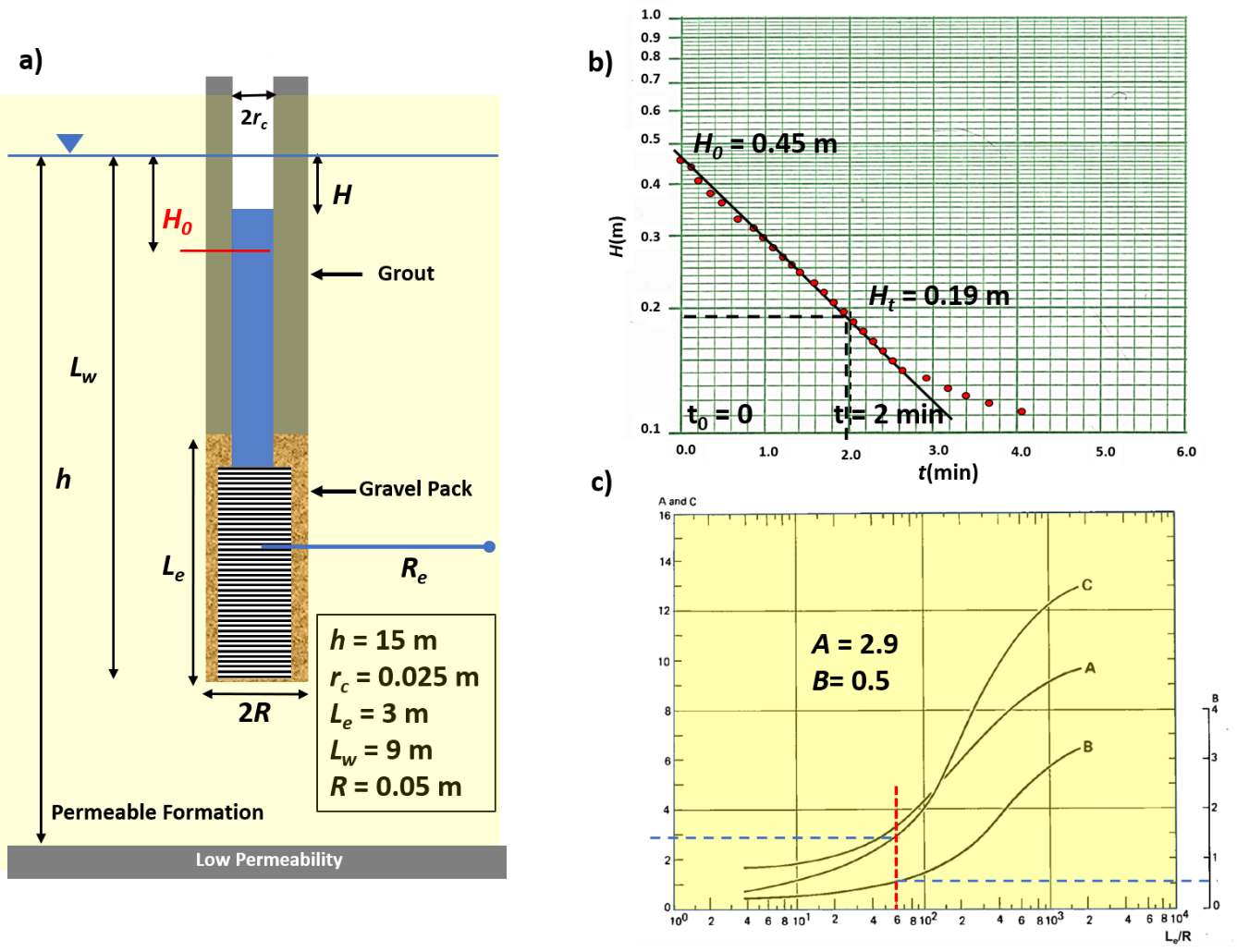
Figure 120 ‑ Conditions under which a slug‑out, rising‑head test, was conducted. a) Parameters of the test well. b) Semi‑log plot of the field data for the log of H versus time. c) Empirical relationships of A, B and C versus Le/R (modified from Kruseman & de Ritter, 2000).
The first step is to estimate ln(Re/R) using Equation (110). As Lw, 9 m, is less than h, 15 m, the constants from Figure 120 are A=2.9 and B=0.5.
[latex]\ln\left( \frac{R_{e}}{R} \right) = \left( \frac{1.1}{\ln\left( \frac{R}{L}_{w} \right)} + (A + B)\ln\left( \frac{\frac{h - L_{w}}{R}}{\frac{L_{e}}{R}} \right) \right)^{- 1} = \left( \frac{1.1}{\ln\left( \frac{0.05\ m}{9\ m} \right)} + (2.9 + 0.5)\ln\left( \frac{\frac{15\ m\ - \ 9\ m}{0.05\ m}}{\frac{3\ m}{0.05m}} \right) \right)^{- 1} = 2.14[/latex]
The K is calculated using Equation (109).
[latex]K = \frac{{r_{c}}^{2}\ln\left( \frac{R_{e}}{R} \right)}{2\ L_{e}t}\ln\frac{H_{0}}{H_{t}} = \frac{{(0.025\ m)}^{2}2.14}{2\ (3\ m)\ 2\ minutes}\ln\frac{0.45\ m}{0.19\ m} = 0.000096\frac{m}{minute}[/latex]
[latex]K = 0.000096\frac{m}{minute}\frac{1440\ minute}{1\ day} = 0.14\frac{m}{day}[/latex]
Cooper‑Bredehoeft‑Papadopulos Slug‑Test Method
The method developed by Cooper and others (1967) is used to assess slug‑test results in wells that fully penetrate a confined aquifer. The method is commonly referred to as the Cooper‑Bredehoeft‑Papadopulos method.
The method requires that the perforated interval of the test well fully penetrates the fully confined geologic unit being tested. It assumes the unit being tested is infinite in lateral extent, isotropic, and homogeneous. Values of T and S are computed. The test configuration and nomenclature are presented in Figure 121.
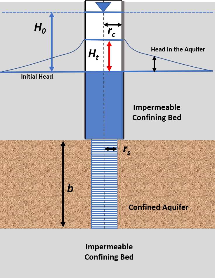
Figure 121 ‑ Slug‑in test configuration and parameters used for the Cooper‑Bredehoeft‑Papadopulos Method. The tightly confined system of thickness b is fully penetrated by the screened interval of radius rs. The casing radius is rc. At the start of the test the water level in the well instantaneously rises to a position H0 above the static water level. The decline of the water level over time is measured as Ht (after Cooper et al., 1967).
Cooper and others (1967) developed a slug‑test analytical solution for the rise or fall of head in a fully penetrating well completed in a totally confined aquifer. Their method includes the general assumptions for the development of analytical solutions for confined aquifers discussed in Sections 6 and 8. Additional assumptions include that the head in the well is static at the beginning of the test and changes instantaneously at t0 = 0; the well diameter is finite, meaning the water stored in the well bore must be considered; in response to an instantaneous head change in the well the rate at which the water flows from or to the well bore (falling‑head or rising‑head test) equals the rate of change of water volume in the well casing; and well loss is negligible (Kruseman & de Ridder, 2000).
The resulting solution is a function F([latex]\alpha[/latex],β) with two variables of integration, α and β (Kruseman & de Ridder, 2000) as shown in Equations (112) and (113).
| [latex]\frac{H_{t}}{H_{0\ }} = F(\alpha,\beta) = \frac{8\alpha}{\pi^{2}}\int_{0}^{\infty}\frac{\exp\left( - \frac{\beta u^{2}}{\alpha} \right)}{u\ f(u,\alpha)}du[/latex] | (112) |
|---|
and
| [latex]f(u,\alpha) = \lbrack uJ_{0}(u) - 2\alpha J_{1}\rbrack^{2} + \lbrack uY_{0}(u) - 2\alpha Y_{1}(u)\rbrack^{2}[/latex] | (113) |
|---|
where:
| Ht | = | head at time t after the maximum head change occurs (L) |
|---|---|---|
| H0 | = | instantaneous change of head at time t0 (L) |
| F(α,β) | = | a function including an integral with variables α and β (dimensionless) |
| J0 and J1 | = | Bessel functions of the first kind, orders 1 and 2 |
| Y0 and Y1 | = | Bessel functions of the second kind, orders 1 and 2 |
The complete definition of the well function is given in Kruseman and de Ridder (2000, p. 239). The variables of integration are defined by Equations (114) and (115).
| [latex]\alpha = \frac{{r_{s}}^{2}S}{{r_{c}}^{2}}[/latex] | (114) | |
|---|---|---|
| [latex]\beta = \frac{Tt}{{r_{c}}^{2}}[/latex] | (115) |
where:
| α | = | parameter abbreviation (dimensionless) |
|---|---|---|
| β | = | parameter abbreviation (dimensionless) |
| rs | = | radius of the screen (L) |
| rc | = | radius of the casing (L) |
| S | = | storativity (dimensionless) |
| T | = | transmissivity (L2T‑1) |
| t | = | time (T) |
The type curves are plotted from tables generated by using various values of α and β (Figure 122 and Figure 123). Additional table values and type curves can be plotted by using the analytical solutions and inputting additional values of β and α. Most often curves are computed using computer‑assisted methods (Section 14.6).
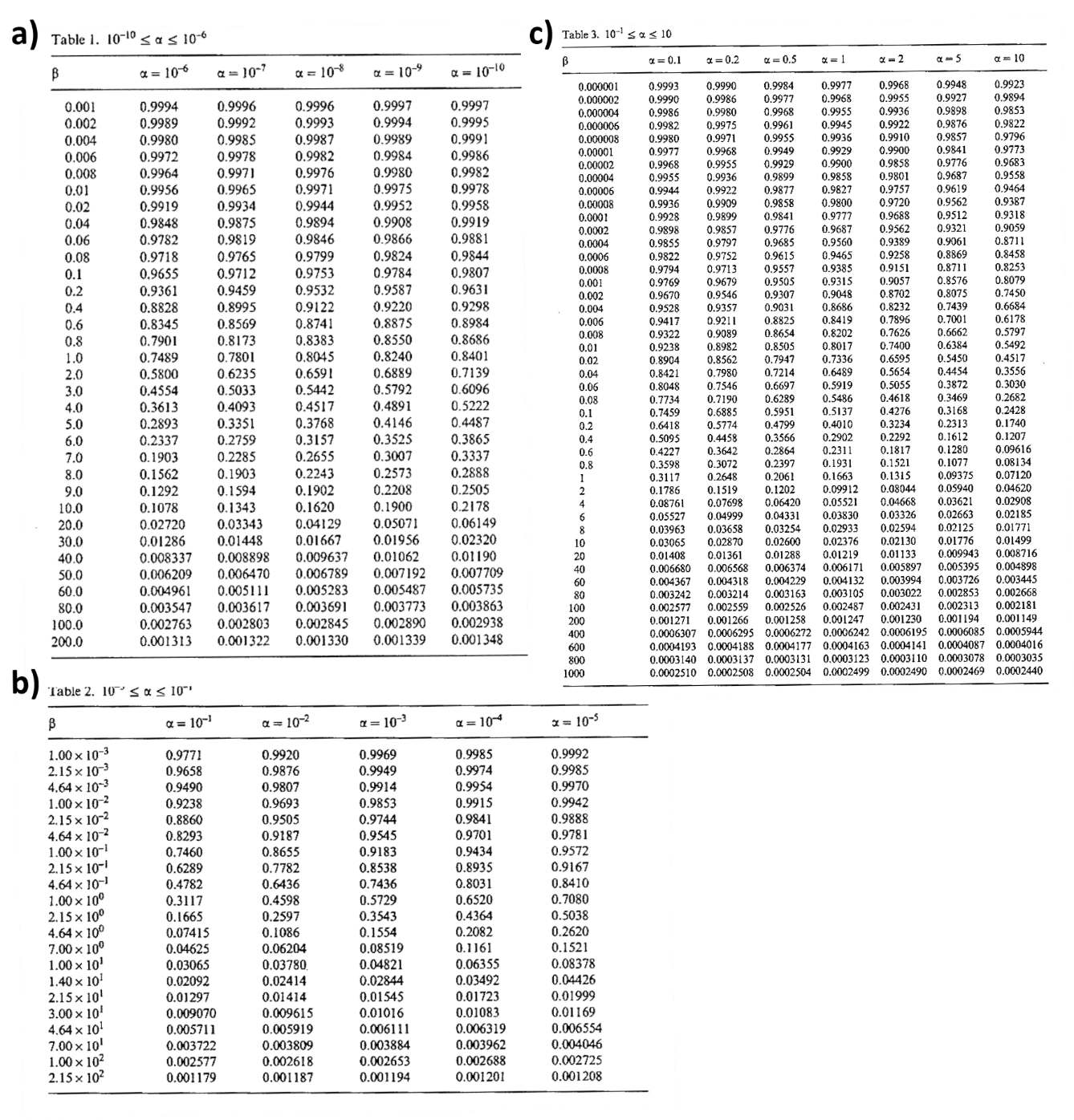
Figure 122 ‑ Tables of the well function F(α,β) values computed for the Cooper‑Bredehoeft‑Papadopulos method analytical solution of slug tests in a totally confined aquifer with a fully penetrating well. a) α from 1×10‑10 to 1×10‑6 and β from 0.001 to 200; b) α from 1×10‑5 to 1×10‑1 and β from 0.001 to 215; c) α from 0.1 to 10 and β from 1×10‑6 to 1000 (Kruseman & de Ritter, 2000).
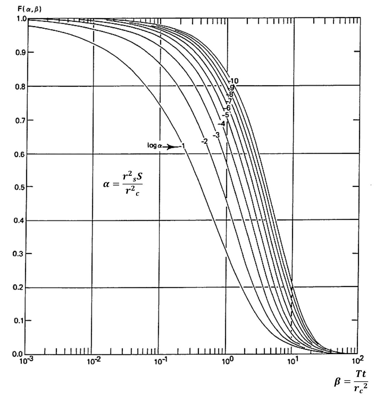
Figure 123 ‑ Type curves for analyzing slug test data for a confined aquifer with a fully penetrating well using the Cooper‑Bredehoeft‑Papadopulos Method. Values of F(α,β) are plotted on the arithmetic vertical scale and β on the horizontal logarithmic scale (modified from Kruseman & de Ritter, 2000).
To analyze slug‑test data for the described confined‑aquifer conditions the field data are plotted as Ht/H0 on the arithmetic vertical axis and the log of t on the horizontal axis. Both the type curves and field data are plotted on the same semi‑log scales, the horizontal axes are kept parallel, and the curves are matched by sliding them horizontally. The plots are not moved vertically. The match point yields values of F(α,β), α, β, Ht/H0, and t (Figure 124). The matched value of α and β are then used to solve for T and S.
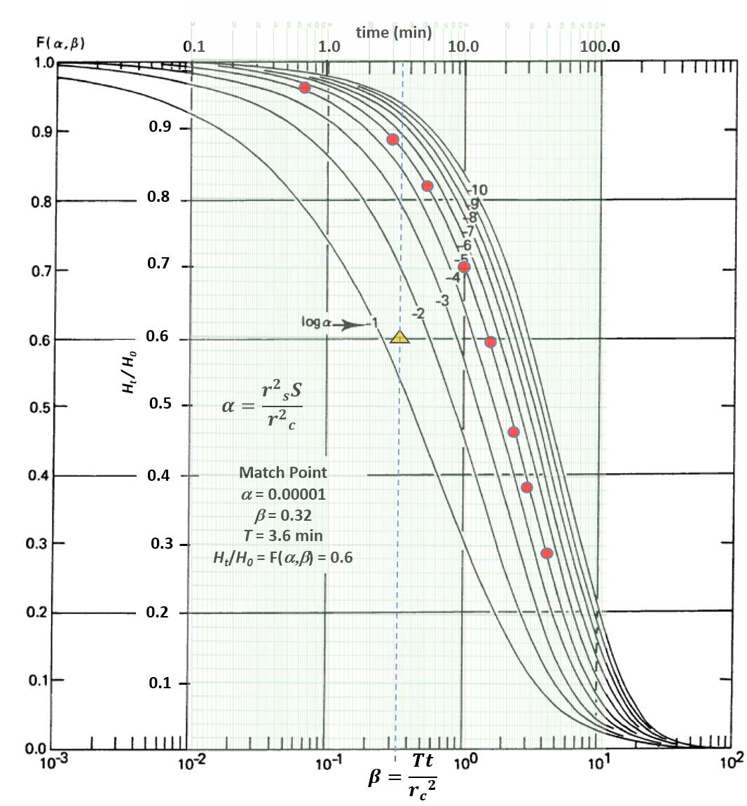
Figure 124 ‑ Cooper‑Bredehoeft‑Papadopulos Method of curve matching. Semi‑log plots of the test data and the type curves are prepared on the same scales. The test data are then moved horizontally keeping the vertical axes values for both plots coincident until the observation data matches one of the curves. A match point is then chosen in the overlapping fields from which values of β and t are derived. a is the value of the curve matched with the field data. For this method the values of Ht/H0 and F(α,β) are equal and not used in the calculation of T and S.
Example
Assume the data presented in Figure 124 represents a falling‑head slug test of a totally confined aquifer that is 30 m thick (b). The well is fully penetrating, and the well radius and screen radius are the same, rs = rc = 10 cm.
The match point yields β = 0.7 at t = 3.6 min and α = 0.00001. Using Equation (115), rearranged to solve for T, yields 2.8 m2/d.
[latex]\beta = \frac{Tt}{{r_{c}}^{2}}[/latex]
[latex]T = \frac{{{\beta r}_{c}}^{2}}{t} = \frac{0.7\ \left( 10\ cm\frac{1\ m}{100\ cm} \right)^{2}}{\left( 3.6\ mimute\frac{1\ d}{1440\ minute} \right)} = \frac{{2.8\ m}^{2}}{d}[/latex]
[latex]K = \frac{T}{b} = \frac{\frac{{2.8\ m}^{2}}{d}}{30\ m} = \frac{0.09\ m}{d}[/latex]
S is computed using Equation (114).
[latex]\alpha = \frac{{r_{s}}^{2}S}{{r_{c}}^{2}}[/latex]
[latex]S = \frac{\alpha{\ r_{c}}^{2}}{{r_{s}}^{2}} = \frac{0.00001{\ (10\ cm)}^{2}}{{\ (10\ cm)}^{2}} = 0.00001[/latex]
KGS Slug Test Method
The Cooper and others (1960) model used to analyze a slug test in a confined aquifer was generalized more recently by Hyder and others (1994). As the principal authors were associated with the Kansas Geological Survey the model is referred to as the KGS model (1994). The KGS method in included here because it is a more general method supported by the software packages.
The KGS method uses a curve‑matching method that is similar to the approach of Cooper and others (1960). It accounts for partial penetration, anisotropy, skin effects and can be used to analyze both confined and unconfined conditions. The model parameters are represented in Figure 125.
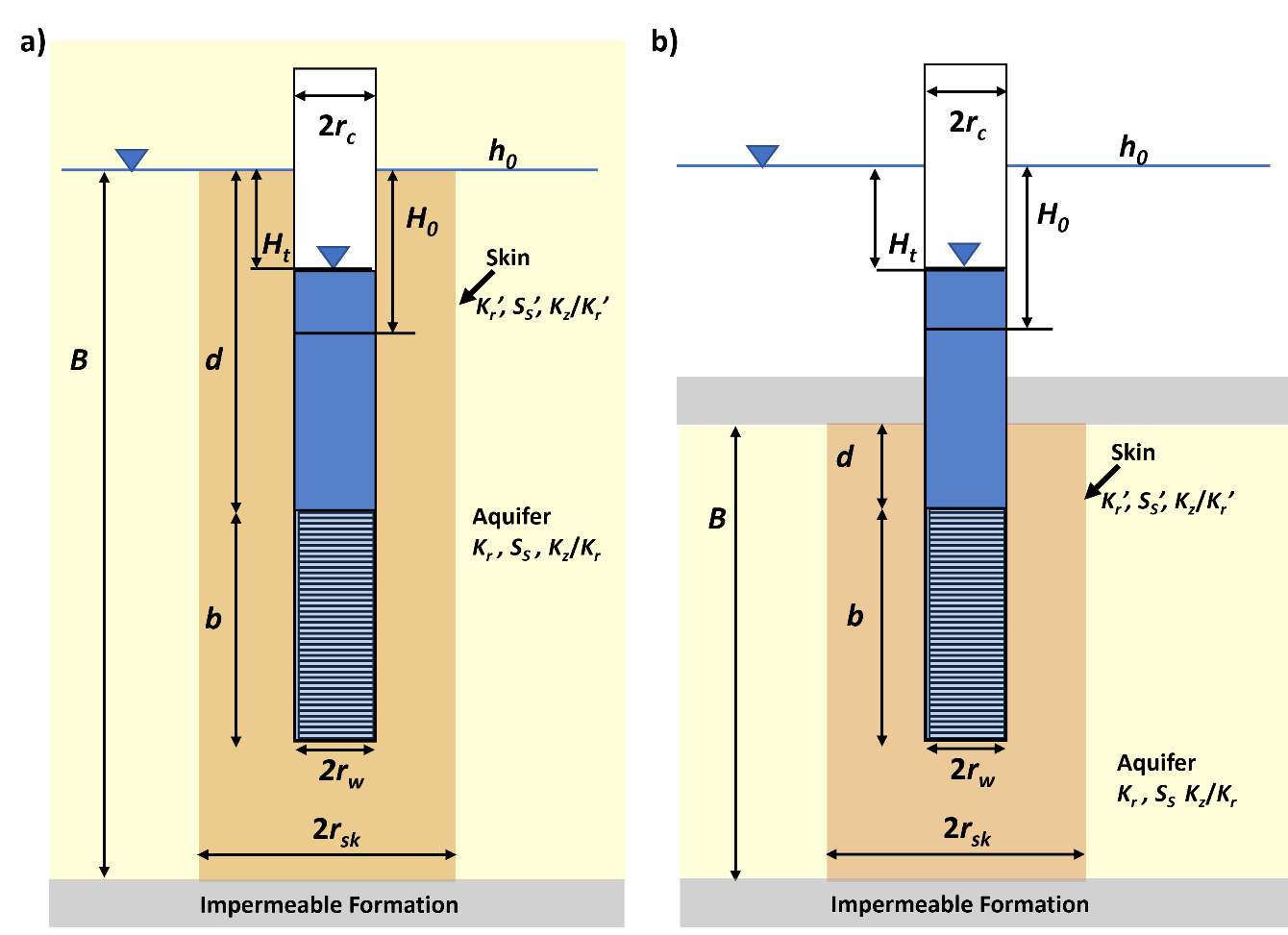
Figure 125 ‑ Schematic of the parameters used in the KGS slug‑test method (Hyder et al., 1994). Gray shading represents impermeable material, yellow shading is the aquifer (Kr, Ss, Kz/Kr), and light orange shading represents a skin effect zone with different hydraulic properties (Kr’, Ss’, Kz/Kr’). H0 is the instantaneous head change from the static (h0) at the beginning of the test and Ht is the head measured from the static at some time during the test. B is the aquifer thickness. d is the length of the blank casing in the aquifer and b is the length of screen. rw is screen radius, rc is the casing radius and rsk is the radius of the skin zone. a) A representation of unconfined conditions. b) A representation of confined conditions.
The analytical solution developed by Hyder and others (1994) is based on the conditions that the aquifer is infinite in extent, homogeneous, and of uniform thickness; the potentiometric surface is initially horizontal; the well is fully or partial penetrating; water‑level change is instantaneous; conditions can be confined or unconfined; and flow is unsteady. Hydraulic anisotropy and skin effects can be accounted for. However, the authors stress that although accounting for specific storage, anisotropy, and skin effect is theoretically possible, the model is rather insensitive to these parameters. The analytical solution is written as shown in Equation (116).
| [latex]\frac{H_{t}}{H_{0}} = F\left( \beta,\alpha,\varphi,\frac{d}{b},\frac{b}{B} \right)[/latex] | (116) |
|---|
where:
| Ht | = | water level in the well at time t (L) |
|---|---|---|
| H0 | = | water level at in the well at the start of the test, at time t0 (L) |
| β | = | KrBt/r2 (dimensionless) |
| α | = | (rw2SsB)/rc2 (dimensionless) |
| ψ | = | (Kz/Kr)0.5/ (b/rw) (dimensionless) |
| B | = | saturated thickness of the aquifer (L) |
| t | = | time (T) |
| Kr | = | radial hydraulic conductivity (LT‑1) |
| rc | = | well‑casing radius (L) |
| rw | = | screen or perforated interval radius (L) |
| Ss | = | aquifer specific storage (L‑1) |
| Kz | = | vertical aquifer hydraulic conductivity (LT‑1) |
| b | = | length of screen or perforated interval (L) |
Type curves are generated by plotting the normalized head (Ht/H0) versus the logarithm of β for field well configuration parameters (ψ,d/b,b/B). An example is presented in Figure 126.
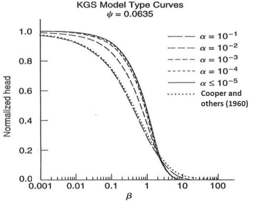
Figure 126 ‑ Type curves for the KGS slug‑test method where ψ = 0.0635. Normalized head values are plotted on the y axis and the logarithm of β on the x axis. Type curves for various values of α are shown. For comparison with the method of Cooper and others (1960), the dotted line equivalent to α=0.1 is presented (Hyder et al., 1994; Butler, 1998).
The field data are plotted as Ht/H0 versus time since the test began and the recovering head at time t is divided by the head at the beginning of the test (Figure 127).
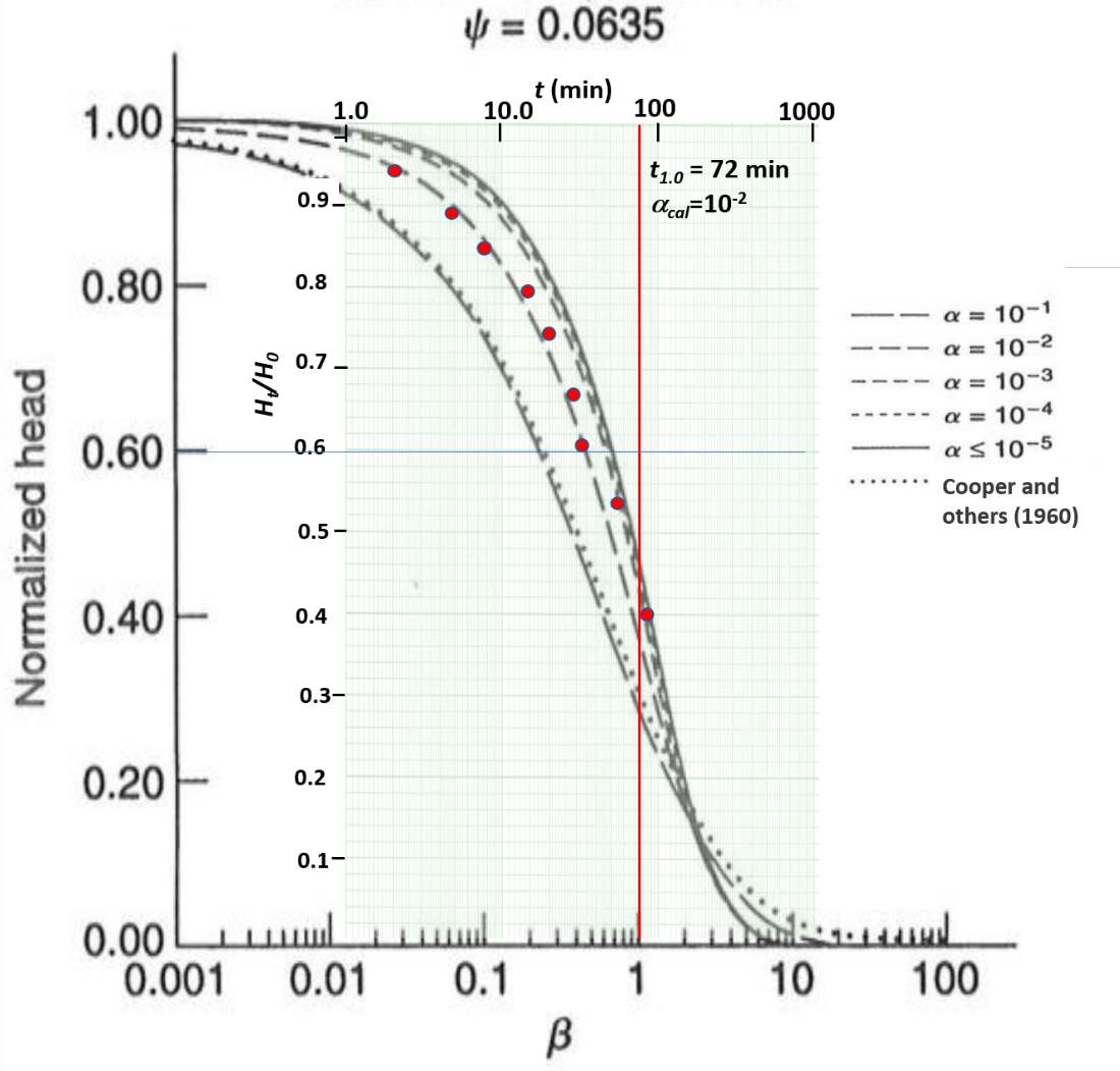
Figure 127 ‑ Example of KGS curve matching. The field data are plotted at the same scale as the type curves as is done when using the method of Cooper and others (1960). The type curve is overlain on the field data and matched to an α curve by sliding the type curve along the x axis. No vertical movement of either graph occurs. Once a curve match is achieved, the field time value (t1.0) corresponding to β=1 is read from the x axis and α is estimated from the matching point (αcal). With these data, the radial hydraulic conductivity is derived from the definition of β.
| [latex]K_{r} = \frac{r_{c}^{2}}{bt_{1.0}}[/latex] | (117) |
|---|
where:
| Kr | = | radial hydraulic conductivity (LT‑1) |
|---|---|---|
| rc | = | well casing radius (L) |
| b | = | length of screen or perforated interval (L) |
| t1.0 | = | time corresponding to β=1.0 for curve match to field data as shown in Figure 127 (Τ) |
Specific storage is computed accounting for partial penetration.
| [latex]S_{s} = \alpha_{cal}\frac{r_{c}^{2}}{r_{w}^{2}b}[/latex] | (118) |
|---|
where:
| Ss | = | specific storage (L‑1) |
|---|---|---|
| αcal | = | α match value |
| rc | = | well casing radius (L) |
| rw | = | screen or perforated interval radius (L) |
| b | = | length of screen or perforated interval (L) |
| t1.0 | = | time corresponding to β=1.0 for curve match to field data as shown in Figure 127 (Τ) |
Example
A slug‑out test is performed on a partially penetrating well in a fine‑grained unconfined system. The well screen and casing radius are 0.0248 m. The well screen is 0.39 m long and partially penetrates the 4 m thick aquifer. No skin effect is identified, and the aquifer is assumed to be isotropic (Kr=Kz). The ψ value is 0.0635 for this well configuration. The radial hydraulic conductivity is calculated from the curve match shown in Figure 127.
Using the curve match and well parameters Kr is calculated assuming Kz/Kr = 1.
[latex]K_{r} = \frac{r_{c}^{2}}{bt_{1.0}}[/latex]
[latex]K_{r} = \frac{{(0.0248\ m)}^{2}}{0.39\ m\ 72\ min\ \frac{1\ d}{1440\ min}} = \frac{0.032\ m}{d}[/latex]
[latex]S_{s} = \alpha_{cal}\frac{r_{c}^{2}}{r_{w}^{2}b}[/latex]
[latex]S_{s} = 0.01\frac{{(0.0248\ m)}^{2}}{{(0.0248\ m)}^{2}\ 0.39\ m} = \ 0.26\ m[/latex]
Limitations of the KGS Method
A comparison study by Ismael (2016) showed that the KGS model (Hyder et al., 1994) provided similar estimates of K to the Hvorslev (1951) method when applied to two unconfined‑aquifer settings. Butler (1998) states that when using the KGS method with a fully penetrating well Ss estimates may not be reliable especially when ψ>0.005. He notes that when using the KGS model, it is “…virtually impossible to estimate the anisotropy ratio in field applications”. He states that a shift in the field data suggesting a decrease in the anisotropy ratio cannot be separated from one caused by a decrease in radial hydraulic conductivity. Butler (1998) suggests anisotropic conditions are better distinguished using multiple‑well slug‑test methods presented in his book and the literature.
As with other curve‑matching methods, software can provide calculations using appropriate well‑configuration type curves and apply automated‑matching methodologies. However, the user needs to specify an initial value for anisotropy, which is often assigned a value of one because it is not known, even though the vertical hydraulic conductivity is typically lower in most materials—a notable exception is loess which often has a higher vertical hydraulic conductivity due to its wind‑blown deposition. Manual fine tuning of the automated computed match improves the parameter estimates as discussed in Section 14.6.