
14.5 Method to Interpret Underdamped Slug Tests
An underdamped‑response of a groundwater system to slug testing is commonly encountered when formational hydraulic conductivity is high. The response to a slug‑in or slug‑out test is oscillatory as shown in Figure 103. The oscillatory behavior of the water level is like that of a damped spring as described in physics books where the force of gravity on a mass hung from a spring and the energy stored in the spring counteract and the motion gradually dissipates as the kinetic energy is converted to thermal energy (e.g., Kreyszig, 1979).
Several authors have developed methods to analyze an underdamped slug test response including van der Kamp (1976), Kipp (1985), Springer and Gelhar, 1991), Wylie and Magnuson (1995), McElwee and Zenner (1998), Zurbuchen and others (2002), Butler (1998), and Butler and others (2003). Butler and Garnett (2000) produced a Kansas Geologic Survey open file report and Butler and others (2003) published a journal article that presents a type‑curve methodology for assessing test results from unconfined and confined formations based on descriptions by Springer and Gelhar (1991) and Butler (1998). They developed two high‑hydraulic conductivity models based on the Bouwer and Rice (1976) and Hvorslev (1951) slug‑test formulations, the high‑K Bouwer and Rice, and the high‑K Hvorslev models (Butler & Garnett, 2000; Butler et al., 2003). Their work utilized spreadsheet models to develop type curves and generate estimates of K. They provide free access to the spreadsheet models on the KGS website↗. The methods are described in the paper by Butler and Garnett (2000) published by the KGS and the journal article by Butler and others (2003). A description of this methodology follows.
Slug testing of high hydraulic conductivity formations (like sand and gravels, and gravels) requires attention to detail as the oscillatory response often occurs over the first few seconds to 10s of seconds of the test. In cases where slug‑displacement volumes are small, and screened intervals long, observable water‑level responses may only last a few seconds. A successful test requires an instantaneous water‑level change and a transducer set to record water‑level variations with a time interval of a fraction of a second if possible. Butler and others (2003) report that the pneumatic air‑displacement method is recommended for head displacement as the release of air pressure at the initiation of the test results is a near‑instantaneous head change (Figure 109, Figure 128). Solid slugs are used when pneumatic test methods are unavailable.
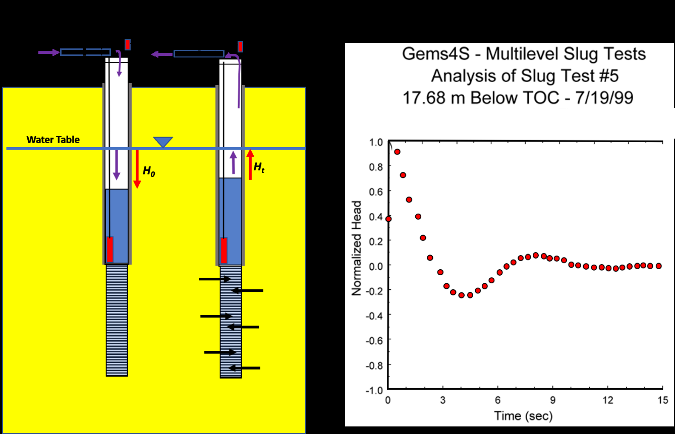
Figure 128 ‑ Pneumatic slug test set up and plot of normalized head change data. An initial static head measurement is taken before the test is initiated. a) Pneumatic slug‑test set up as described in Figure 108. The casing is capped and fitted with a valve, airline, and gauge and/or pressure transducer. A second transducer is placed below the maximum water level, H0. The water table is depressed by pressurizing the water column in the sealed casing. The valve is closed and H0 computed from the pressure gage reading or a cap mounted pressure transducer (small red rectangle). At time zero the valve is opened, and the water level is allowed to recover. A transducer (large vertical red rectangle) in the well records the water level response. b) Plot of normalized slug test head data (red dots), Ht/H0. The normalized head data are plotted on an arithmetic scale with a zero value (static‑fully recovered water level), and positive and negative values centered on the static water level.
Prior to beginning the slug test a static water level is measured using steel or electronic water‑level tape. At the initiation of the test the well is capped, and the casing pressurized. The displacement value H0 is estimated from the pressure gage or cap transducer reading (air pressure depressing the water level). It is recommended that multiple tests be conducted using different displacements, H0. Values of K should not be dependent on H0. Butler and Garnett (2000) and Butler and others (2003) report that the depth of the transducer below the static level is important. They found that when the well transducer was located within 0.5 m of the static water level the resulting measured maximum value of Ht/H0 was 0.9 or higher. They suggest that if the test is run and the recorded maximum normalized head is less than 0.9, the test should be repeated with the transducer raised to a new position closer to the static water level. Of course, the transducer must be below the water level (H0) measured at the beginning of the test. It is also important that the transducer sensitivity range, accuracy, and recording interval meet the slug‑test design.
Development of Type‑Curve Equations
Butler (1996), Butler and Garnett (2000), and Butler and others (2003) provide the theory and equations used to develop type curves for analysis of oscillatory data. The methodology is applicable to unconfined and confined systems. An example of data analysis by this method follows.
Type curves based on CD, a dimensionless damping factor, td dimensionless time, and the normalized water‑level deviation, wd, are generated using the overdamped type‑curve equations based on the damped‑spring solution (Kreyszig, 1979) as shown in Equations (119), (120), and (121). The equations express the relationship between the dimensionless normalized head wd at dimensionless time td (i.e., w(td)) for various values of the dimensionless damping parameter CD. The Le term is calculated as part of the curve matching process (i.e., Le = (t*/td*)2g, where * denotes a curve match value and g is the acceleration due to gravity (modified from Butler and & Garnett, 2000; Butler et al., 2003).
| [latex]w_{d}(t_{d}) = e^{–\frac{C_{D}}{2}t_{d}}\left\lbrack cos(\omega_{d}t_{d}) + \frac{C_{D}}{2\omega_{d}}\sin\left( \omega_{d}t_{d} \right) \right\rbrack,\ C_{D} < 2[/latex] | (119) | |
|---|---|---|
| [latex]w_{d}\left( t_{d} \right) = e^{–t_{d}}\left\lbrack 1 + t_{d} \right\rbrack,\ C_{D} = 2[/latex] | (120) | |
| [latex]w_{d}\left( t_{d} \right) = \left( \frac{1}{\beta_{1} - \beta_{2}} \right)\left( \beta_{1}e^{\beta_{2}t_{d\ –\ }}\beta_{2}e^{\beta_{1}t_{d}} \right),\ C_{D} > 2[/latex] | (121) |
where:
| CD | = | damping parameter (dimensionless) |
|---|---|---|
| g | = | acceleration of gravity (LT‑2) |
| H0 | = | change in water level initiating a slug test (initial displacement (L) |
| Le | = | effective length of water column in well calculated as part of the curve matching process (i.e., Le = (t*/td*)2g, where * denotes a curve match value and g is the acceleration due to gravity (L) |
| td | = | time parameter ((g/Le )0.5)t) where t = time (dimensionless) |
| w | = | deviation of water level from static level in well (L) |
| wd | = | normalized water‑level deviation (T) |
| ωd | = | frequency parameter (|1– (CD/2)2|0.5) (dimensionless) |
| β1 | = | – (CD/2) – ωd (dimensionless) |
| β2 | = | – (CD/2) + ωd (dimensionless) |
For values of wd, td, and CD type curves are generated and plotted on an arithmetic scale with wd = 0 representing the static normalized water level (Figure 129). The slug‑test data are plotted on the same vertical scale as the type curves being utilized (Figure 130).
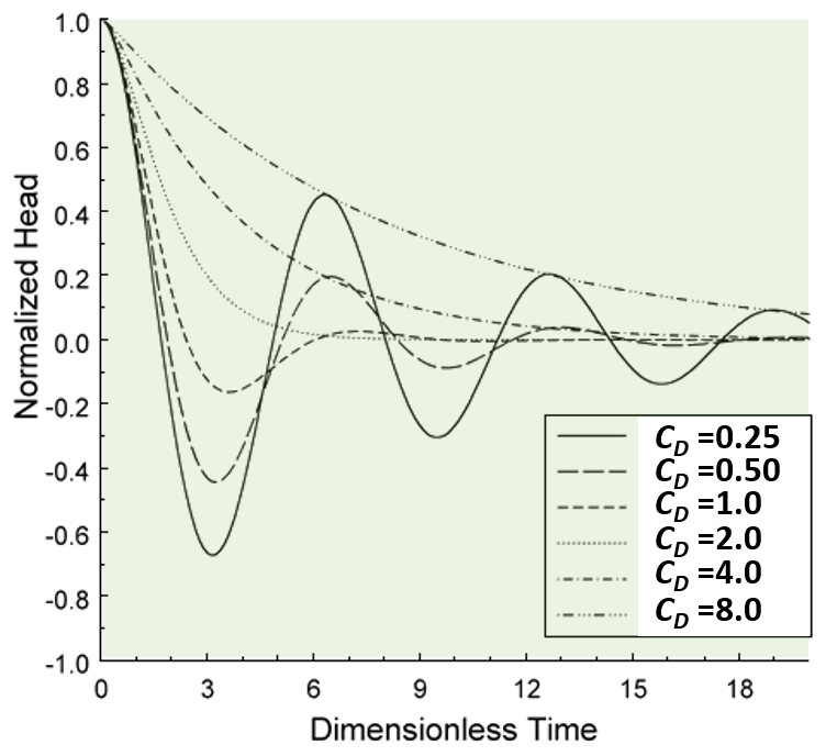
Figure 129 ‑ Type curves used to analyze overdamped slug test responses. The arithmetic plot of normalized head (wd) versus dimensionless time (td) for various dampening parameter values CD (Butler & Garnett, 2000).
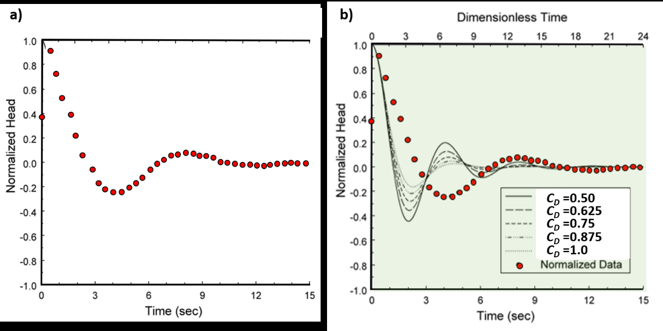
Figure 130 ‑ Example from Butler and Garnett (2000) of slug test GEMS4S conducted at the Geohydrological Experimental and Monitoring Site (GEMS) in Douglas County Kansas, USA. a) Slug‑test results shown in red dots plotted as normalized head versus time at the same vertical scale as the type curves. b) Slug‑test data superposed on the type curves representing curves generated for the dimensional damping parameter CD between 0.50 and 1.0. This superposition is shown to illustrate the process. Field data and type curves are adjusted to obtain a match. The base x axis is the slug‑test time, and the upper x axis is the type‑curve dimensionless time. The illustrated type curves and data do not match in this figure (Butler & Garnett (2000).
The slug‑test data are superposed on the type‑curve plot. The normalized head and dimensionless time scales are identical. The test time scale (x axis on Figure 130) is the slug‑test time data, and the upper x axis is the type‑curve dimensionless time axis. To obtain the best match between the field data and type curve, the field‑data plot remains unchanged as the type‑curve plot is stretched and contracted horizontally, attempting to generate the best match with the CD values. The scale of the vertical axes is not changed. Once a match is determined, values of CD*, td*, and t* (* is used to designate match values) are generated and used to solve for K. The Excel® spreadsheet software provided by Butler and Garnett (2000) kgs.ku.edu/Hydro/Publications/OFR00_40/kgs.ku.edu/Hydro/Publications/OFR00_40↗ generates a family of type curves that most closely match the slug‑test data and facilitates the fitting process. Iterative adjustment by the user is relied upon to generate visual matches between the data and type curves. Butler and others (2003) describe the use of the type‑curve generator spreadsheet and high‑K estimator spreadsheets. The Butler and Garnett (2000) fitting process and results for their example problem are shown in Figure 131.
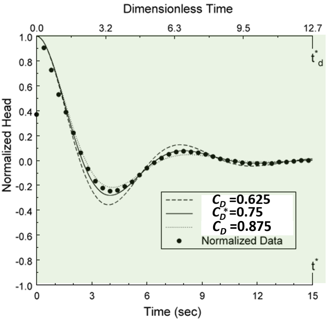
Figure 131 ‑ Final match of slug‑test data (black dots) presented by Butler and Garnett (2000). Only the CD values that most closely match the field data are shown with a best match of CD*=0.75 in this example. The additional match values are td* = 12.7, and the corresponding slug‑test data time t* = 15 sec (Butler & Garnett, 2000).
Butler and others (2003) note that matches can be achieved because the value td controls the period (duration), and CD controls the degree of curvature or oscillatory behavior. The curve match for the example shown in Figure 130 provides values of CD* = 0.75, td* = 12.7 and t* = 15 sec (* denotes these as match values). These values are used to solve for K using the Unconfined‑High‑K Bouwer and Rice model (Springer & Gelhar, 1991) or the Confined‑High‑K Hvorslev model (Butler, 1998). The High‑K models are contained in the High‑K Estimator spreadsheet that also requires well construction data, and an estimate of the effective length of the water column (Le).
Unconfined‑High‑K Bouwer and Rice Model
The Unconfined‑high‑K Bouwer and Rice Model is based on the work of Springer and Gelhar (1991) as presented by Butler and others (2003) and shown here as Equation (122).
| [latex]K_{r} = \frac{t_{d}^{*}}{t^{*}}\frac{{r_{c}}^{2}\ln\left( \frac{R_{e}}{r_{s}} \right)}{2\ bC_{D}^{*}}[/latex] | (122) |
|---|
where:
| td* | = | curve match time (dimensionless) |
|---|---|---|
| t* | = | slug‑test curve match time (T) |
| rc | = | well‑casing radius corrected for the radius of the transducer cable (L) |
| rs | = | radius of the well screen or borehole in isotropic aquifer, rs (Kz/Kr)0.5 for anisotropic systems (L) |
| Kr | = | radial hydraulic conductivity (LT‑1) |
| Re | = | effective radius of the slug test is computed as ln(Re/rs) from Equation (110) or (111) where h is the aquifer thickness (units of L) and Lw is the distance from the bottom of the well screen to the water table (units of L), and Le is the effective length of the well screen (b as defined here) (units of L). Figure 121 provides definitions of these parameters. (dimensionless) |
| b | = | screen length (L) |
| CD* | = | match of dampening parameter (dimensionless) |
The High‑K Bouwer and Rice model can be used when the base of the well screen is in contact with an impermeable boundary (lower boundary). The Le parameter used to compute Re is defined in Figure 116 as the effective length of the well screen. It is not the same Le factor used in the type‑curve calculations of Equations (119), (120), and (121) as defined in the list of parameters below Equation (121). The High‑K‑Estimator spreadsheet assists in computing the Kr value.
Confined – High‑K Hvorslev Model
The High‑K Hvorslev model was developed by Butler and others (2003). It is defined by Equation (123).
| [latex]K_{r} = \left( \frac{t_{d}^{*}}{t^{*}} \right)\frac{{r_{c}}^{2}\ln\left( \frac{b}{2r_{s}} + \left( 1 + \left( \frac{b}{{2r}_{s}} \right)^{2} \right)^{0.5} \right)}{2\ bC_{D}^{*}}[/latex] | (123) |
|---|
where:
| td* | = | curve match time (dimensionless) |
|---|---|---|
| t* | = | slug‑test curve match time (T) |
| rc | = | well‑casing radius corrected for the radius of the transducer cable (L) |
| rs | = | radius of the well screen or borehole in isotropic aquifer, rs (Kz/Kr)0.5 for anisotropic systems (L) |
| Kr | = | radial hydraulic conductivity (LT‑1) |
| b | = | screen length (L) |
| CD* | = | match of dampening parameter (dimensionless) |
The High‑K Hvorslev model does not represent conditions where the bottom of the casing is adjacent to an impermeable bottom boundary. Butler and others (2003) state that if this condition occurs the term 2rs in the numerator of Equation (123) should be replace with rs. They state that corrections for small‑diameter wells can also be incorporated.
Example
A pneumatic slug test was performed in a high hydraulic conductivity, isotropic, confined aquifer as shown in Figure 132.
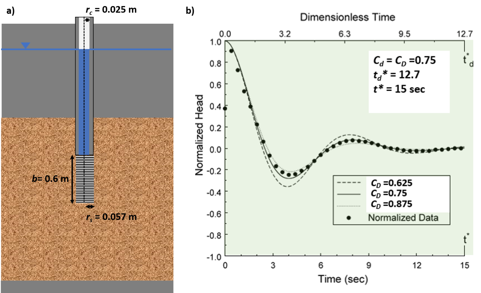
Figure 132 ‑ Set up for a slug test of an isotropic and homogenous sand and gravel confined aquifer and a hypothetical plot of the slug‑test results. a) Well configuration. b) Normalized slug‑test results and curve‑match parameters.
The slug‑test results were normalized and curve matched to the type curves shown in Figure 128. Parameters derived from the type‑curve match are CD = 0.75, td* = 12.7 and t* = 15 sec. The formation is confined so the High‑K Hvorslev Model is applied.
[latex]\begin{aligned} K_{r} &= \left( \frac{t_{d}^{*}}{t^{*}} \right)\frac{r_{c}^{2}\ln\left( \frac{b}{2r_{s}} + \left( 1 + \left( \frac{b}{2r_{s}} \right)^{2} \right)^{0.5} \right)}{2\, b C_{D}^{*}} \\ &= \left( \frac{12.7\,\text{s}}{15\,\text{s}} \right)\frac{(0.025\,\text{m})^{2}\ln\left( \frac{0.6\,\text{m}}{2(0.057\,\text{m})} + \left( 1 + \left( \frac{0.6\,\text{m}}{2(0.057\,\text{m})} \right)^{2} \right)^{0.5} \right)}{2\,(0.6\,\text{m})\,(0.75)} = 0.0014\,\frac{\text{m}}{\text{s}} \end{aligned}[/latex]
[latex]K_{r} = 0.0014\,\frac{\text{m}}{\text{s}}\,\frac{86400\,\text{s}}{\text{d}} = 121\,\frac{\text{m}}{\text{d}}[/latex]
Transitional Slug‑Test Responses
The curve matching methods described above have also been applied to non‑oscillatory slug test responses in highly conductive settings. Results may show a mix of responses. These are referred to as transitional slug test data sets because conditions show a system is acting partly as overdamp and partly as undamped (Figure 103). Butler and others (2003) provide an example of a set of curves derived from the packer test of an interval of a highly conductive aquifer. The data are plotted and then the curve‑matching methodology and Kr calculations are performed. The authors conclude that the underdamped curve‑matching methods and equations provided good estimates of formational properties when hydraulic conductivity values are high. When curve‑matching results were compared to values computed using the conventional overdamped Hvorslev equation method (straight‑line approach) the conventional method produced values that were 13 percent higher than those derived from underdamped curve matching. The authors concluded that when the values of CD were greater than three, conventional underdamped methods provided reasonable values.