
15.2 Testing Methods and Analyses
Packer testing is most frequently applied to boreholes in rock. Testing methods can also examine bulk properties and properties of individual fractures. The work of Quinn and others (2012) is comprehensive reference on borehole testing in fractured rock and provides details on a versatile straddle‑packer system they developed to provide transmissivity estimates. They list four types of hydraulic tests used in porous media that are commonly applied to fractured‑rock boreholes. These are also applicable to some screened boreholes in good communication with the undisturbed formation (Figure 133). Tests include constant‑head step test, instantaneous slug, constant‑rate pumping, and recovery after constant‑rate pumping. In some settings where groundwater‑velocity data are desired, borehole‑dilution methods that circulate a tracer in the packed‑off section of the borehole are used (e.g., Maldaner et al., 2018). Slug, constant‑rate pumping, and constant‑head injection/withdrawal tests are discussed here. Refer to Quinn and others (2012) for application of other methods.
The packer‑test records should include a drillers log, borehole configuration, the dimensions of the test interval, top and bottom elevations of the packers, time and water‑level change data, and the start and stop times. A transducer system is usually used to monitor heads in the test zone. When data loggers are connected to an onsite recording and visualization system, real‑time head changes and flow rates can be observed.
Packer‑isolated sections of a borehole can be tested using standard slug‑test methods described in Section 14, pumping tests for single wells presented in Section 12, and constant‑head injection/withdrawal, step‑rate injection, and drill‑stem tests described in this section.
Slug Tests
A single‑ or dual‑packer system can be used to isolate a zone of interest such that a rising‑ or falling‑head slug test can be executed. A transducer located in the packed‑off zone is installed and records water‑level changes with time. As described in Section 14, the head is instantaneously raised or lowered, and the response of the recovering head is observed. Standard slug‑test analysis methods for a given formation type (unconfined or confined) can be used to analyze the data as described in Section 14.
Constant‑Rate Pumping Tests
When a pump is installed between a double packer or below a single packer, a constant‑discharge aquifer test can be conducted, and T values can be approximated. As observation wells are rarely used, estimates of S are usually poor as explained in Section 12. Transient or steady‑state testing can be performed. Most often the test will be conducted and analyzed as a single‑well test. Analyses methods have been described previously in Sections 7 through 10 and Section 12.
Constant‑Head Injection/Withdrawal Test
This section describes how a constant‑head injection test is performed using a dual‑packer system. Lapcevic and others (1999) provide a complete discussion of constant‑head testing methods.
A constant‑head injection/withdrawal test (also referred to as a Lugeon test or constant‑pressure test) injects or withdraws water under a constant head to or from a packed‑off test interval until a constant‑flow rate is achieved. This simulates steady‑state conditions (Ziegler, 1976). To achieve a constant‑flow rate at a constant head, water could be pumped into the test interval, however, when permeabilities are low, flow rates may be difficult to maintain. Lapcevic and others (1999) report that more commonly a series of water‑filled tanks of varying diameters pressurized with nitrogen are used to maintain constant‑ (and sometimes very‑low) flow rates (Figure 135). Manometers are attached to each tank to measure the tank’s level and the constant head is maintained by a control panel. The flow rate is measured by monitoring the rate of change of the manometer level in each tank with the pressure held constant as the tanks empty. Lapcevic and others (1999) report that this set up generates a wide range of flow rates such that zone transmissivities ranging from 1×10‑10 to 1×10‑3 m2/s can be measured. They recommend that multiple tests should be conducted by increasing the pressure used during each test.
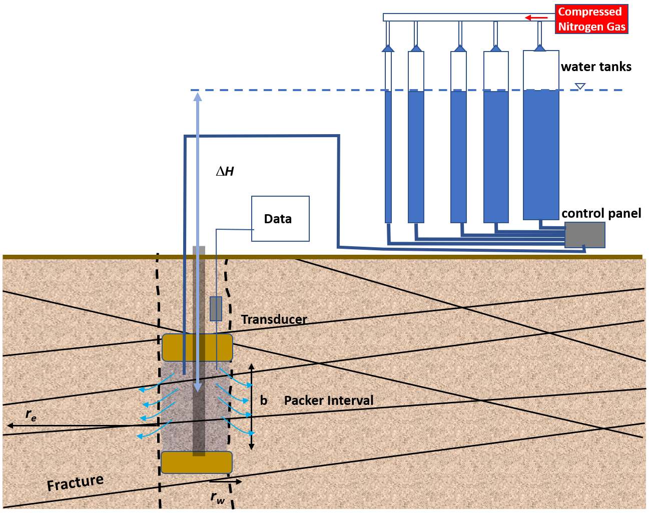
Figure 135 ‑ Set‑up of a constant‑head injection test using multiple tanks to maintain a constant head and flow rate. A constant head is maintained between the packer interval and the pressurized water tanks (∆H). The dashed cross section of a borehole is displayed with two packers isolating a test zone (b). Pressurized nitrogen gas is used to empty the tanks at a constant rate. rw is the radius of the borehole and re is the radius of influence of the test (modified from Lapcevic et al., 1999).
Analyzing Injection/Withdrawal Test Results
The constant‑head injection/withdrawal test is run until the flow rate is no longer changing. The interval transmissivity can be estimated using the Thiem equation for a confined system as shown in Equation (124). It is assumed that purely radial flow is occurring from the packed off interval.
| [latex]T = \frac{Q}{2\ \pi\ \mathrm{\Delta}H\ }\ln\left( \frac{r_{e}}{r_{w}} \right)[/latex] | (124) |
|---|
where:
| T | = | transmissivity (Kb where b is the interval thickness) (L2T‑1) |
|---|---|---|
| Q | = | constant discharge (L3T‑1) |
| ∆H | = | difference in hydraulic head (L) |
| re | = | radius of influence (L) |
| rw | = | radius of the borehole (L) |
The radius of influence is the extent that injection test affects conditions in the material surrounding the test zone. Lapcevic and others (1999) note that re is often assumed to be 10 to 15 m (Bliss & Ruston, 1984). The T calculation is not very sensitive to re as shown by Equation (124) where re is divided by rw and then the natural log of this ratio is computed (Doe & Remer, 1980).
Example
A 4‑m section (b) of a 0.1‑m diameter borehole in a fractured sandstone is isolated by a straddle‑packer system (two packers). An injection test is conducted where the head difference is 5 m, and the steady‑state flow rate is 1 m3/d. The transmissivity (Kb) of the test zone is computed using Equation (124). The radius of influence (re) is assumed to be 12 m.
[latex]T = \frac{Q}{2\ \pi\ \mathrm{\Delta}H\ }\ln\left( \frac{r_{e}}{r_{w}} \right) = \frac{1\frac{m^{3}}{d}}{2\ (3.14)\ 5\ m\ }\ln\left( \frac{12\ m}{0.05\ m} \right) = 0.174\frac{m^{2}}{d}[/latex]
The horizontal hydraulic conductivity is then equal to T/b = 0.174 m2/d/4m = 0.044 m/d. Zones with individual or several fractures can be represented as an equivalent single fracture using an equivalent individual fracture aperture, 2beq. This can be computed from the zone T value (Equation (124)) by applying the cubic law (e.g., Lapcevic et al., 1999) as shown in Equation (125).
| [latex]2b_{eq} = \left( \frac{T12\mu}{\gamma} \right)0.33[/latex] | (125) |
|---|
where:
| 2beq | = | equivalent fracture aperture (L) |
|---|---|---|
| T | = | transmissivity (L2T‑1) |
| μ | = | viscosity of water (MTL‑1) |
| γ | = | specific weight of water (MT2L‑2) |
Step‑Rate Injection Test (Lugeon Test)
Lugeon tests are commonly performed in geotechnical or underground‑mining applications to estimate the hydraulic conductivity and flow regime of a specific test interval. The test method was pioneered by Maurice Lugeon (1933) and later described by Houlsby (1976). It is based on observing the response of the test zone to inflow rate of injected water as the water pressure in the zone increases and decreases. The test set up is presented in Figure 136.
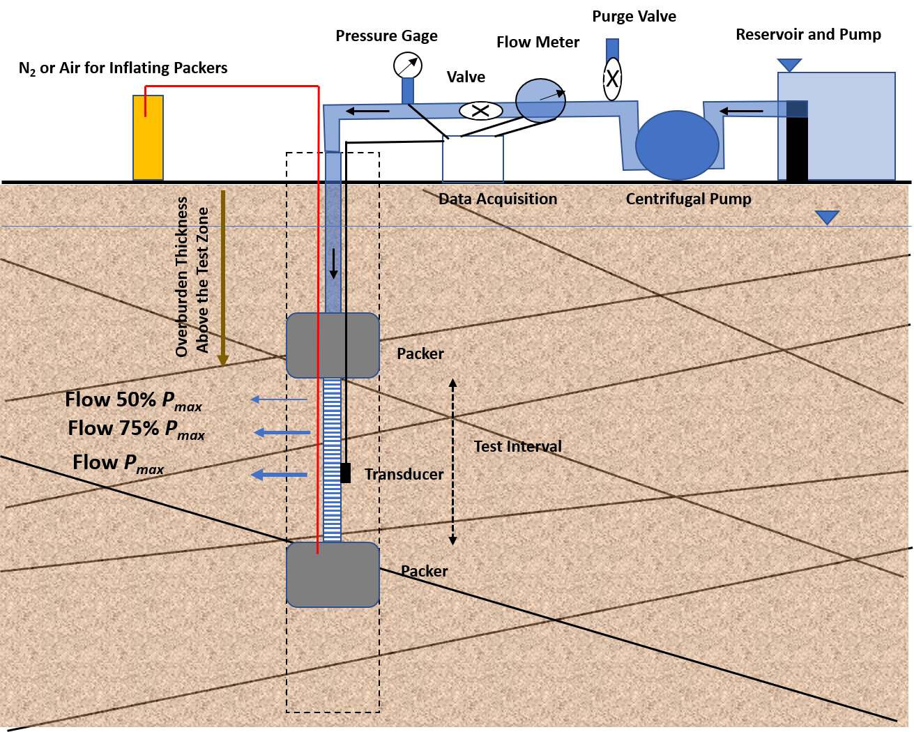
Figure 136 ‑ Schematic set up of a Lugeon test. A dual‑packer system inflated with gas isolates the test zone. The injection test uses water from a reservoir and a pump to pressurize the system and inject water into the test zone. The data collected are the inflow rate at a given pressure over time after rate stabilization. The maximum pressure, Pmax, is computed based on the thickness of overburden overlying the test interval multiplied by 1 pound per square inch per foot (2.26×10⁴ pascals/m). Flow rates at pressures of 50, 75 and 100 percent of Pmax are determined and applied during the test; then the pressures are sequentially lowered back to 50 percent and flow rates recorded again for each interval.
The test is conducted using five stages of water pressure injection. Steps 1 through 3 increase pressure while steps 4 and 5 duplicate the pressure of steps 2 and 1, respectively. The five‑step pressure ‘loop’ allows for interpretation of the flow regime and aids in selection of the most representative hydraulic conductivity value (Quiñones‑Rozo, 2010).
The maximum injection pressure (Pmax) is determined prior to starting the test. Pmax must not exceed the confinement stress in the test interval to avoid hydraulic fracturing. Pmax is typically estimated at 1 pound per square inch (psi) per foot of overburden above the test interval (6,895 Pascal = 1 psi). For example, a Pmax of 200 psi (1.38 MPa) would be appropriate for a test interval located from 61 to 67 m (200 to 220 ft) below ground surface. The vertical thickness of overburden above the test interval is used to calculate Pmax in an angled borehole or for a test conducted beneath a sloping terrain. Pmax represents the highest injection pressure (step 3) and steps 1, 2, 4, and 5 represent multiples of Pmax as shown in Figure 137 (Quiñones‑Rozo, 2010).
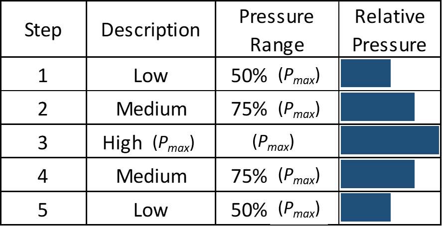
Figure 137 ‑ Five pressure steps used in a Lugeon test. Pmax is the maximum pressure computed as 1 psi per foot of overburden above the test zone (2.26×10⁴ pascals per meter of overburden above the test zone). After step rates have stabilized, the total flow rate is measured every minute over a 10 min interval and the flow rate is determined by averaging the values (Quiñones‑Rozo, 2010).
Water pressure and flow rate are recorded during each step of the test using a totalizing flowmeter, pressure gage/sensor, and timer. A purge valve on the injection system is used to vent excess pressure from the injection pump which controls the injection pressure into the test interval (Figure 135). After establishing a constant‑flow rate, each stage is typically run for 10 minutes. Pressure and totalizing flowmeter readings are recorded each minute, and the total ‘take’ (inflow volume) of the test interval is calculated in liters for each step. The average flow rate is computed from the step data. A hydraulic conductivity value is calculated for each step, expressed as an empirical Lugeon value, which is defined as the hydraulic conductivity required to achieve a flow rate of 1 liter per minute per meter of test interval under a reference water pressure equal to 1 MPa.
Lugeon tests are analyzed based on the total injection pressure and flow during a given step. One Lugeon is equivalent to 1.3 x 10‑5 centimeters per second under homogenous and isotropic conditions (Quiñones‑Rozo, 2010). Separate Lugeon values are calculated for each step using Equation (126).
| [latex]Lugeon\ Value = \ \alpha\ \frac{q}{L}\ \frac{P_{0}}{P}[/latex] | (126) |
|---|
where:
| Lugeon | = | reflects hydraulic conductivity of 1.3 x 10‑5 centimeters per second when determined under homogenous, isotropic conditions |
|---|---|---|
| α | = | dimensionless unit‑conversion factor (1 for SI units which would be in liters per minute, meters, and megapascals) |
| q | = | average flow rate from a single step (in liters per minute) |
| L | = | length of test interval (in meters) |
| P0 | = | reference pressure, which is defined as 1 megapascal |
| P | = | total pressure head above static pressure (i.e., injection pressure + pressure head + frictional losses) |
Houlsby (1976) developed a method to select a representative Lugeon value or equivalent hydraulic conductivity to represent the test interval using the observed patterns of Lugeon values. His method uses a bar graph of Lugeon values calculated for each step. The test values are matched to a pattern, and a method to generate a representative hydraulic conductivity value is selected. The patterns are labeled as representing flow regimes that include (1) laminar flow, (2) turbulent flow, (3) dilation, (4) wash‑out, or (5) void filling. Each regime is described in the caption of Figure 138.
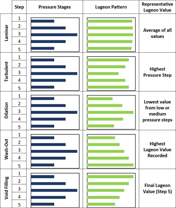
Figure 138 ‑ Lugeon‑test patterns and flow‑regime interpretation (Houlsby, 1976). The pressure stages are the same for each Lugeon pattern. However, the calculation of a representative hydraulic conductivity value is dependent on the pattern of test Lugeon values. (1) Laminar Flow – All Lugeon values for each step are similar, therefore laminar flow is occurring. The representative value is the average of all five steps. (2) Turbulent flow – The lowest Lugeon value occurs at the highest pressure, therefore turbulent flow is occurring. The representative value is the Lugeon value for the highest pressure. (3) Dilation – The highest Lugeon value occurs at the highest pressure, therefore fracture dilation is occurring at high pressure. The representative value is the average of the low pressure (1,5) or medium pressure (2,4) steps. (4) Wash‑Out – Lugeon values increase with each step regardless of pressure, therefore gouge or weathered minerals are washing out of fractures. The representative Lugeon value is the highest observed value unless special conditions dictate otherwise. (5) Void Filling – Lugeon Values decrease with each step regardless of pressure, therefore gouge or weathered minerals are filling in small aperture fractures. The representative value is the Lugeon value for the lowest pressure.
Example
A 11.6‑m long test section of borehole in a fractured sandstone is isolated by a straddle‑packer system (two packers). The first Lugeon test step is conducted for 10 minutes, has an average total head pressure above static of 0.084 megapascals (MPa) and the formation takes a total of 390 liters throughout the step. Using Equation (126) with an SI unit conversion factor of one, a total head of 0.084 MPa, and an average flow rate of 39 liters per minute yields 40 Lugeons.
[latex]Lugeon\ Value = \alpha\ \frac{q}{L}\ \frac{P_{0}}{P} = \ 1\ \frac{39\frac{L}{\min}}{11.6\ m}\ \frac{1\ MPa}{0.084\ MPa} = 40\ Lugeons[/latex]
A Lugeon value of 40 is approximately 5.2 x 10‑4 cm/s. As indicated in the parameter definitions for Equation (126), one Lugeon value is equivalent to 1.3 x 10‑5 centimeters per second under homogenous and isotropic conditions (Quiñones‑Rozo 2010).
The software program AquiferTest V12 provides methods to interpret Lugeon‑test results. The user’s manual provides details on methods and data requirements (Waterloo Hydrogeologic, 2021).
Drill‑Stem Test
Estimates of horizontal hydraulic conductivity using a packed‑off interval of a borehole have been of interest to the petroleum industry for many years (e.g., Mathews & Russel, 1967; Earlougher, 1977). The drill‑stem test procedure is also applicable to the characterization of some confined hydrogeologic settings.
Conceptually, a drill‑stem test involves outfitting the drill stem with a test apparatus within the interval of interest that has packers, valves, and pressure‑monitoring systems. The packer system is used to isolate a section of borehole. Valves are opened at the start of the test and fluid from the packer zone flows into the drill stem for a period of time. Then the valve is closed. The pressure system monitors the starting formational pressures and the recovery pressures after the value is closed. A discharge rate is computed from the rate that the volume of water fills the drill stem once the test is initiated. Analyses of the data are achieved by using recovery theory once the valve system is closed. Domenico and Schwartz (1998) have a brief discussion of the method and data analysis. Additional, detail and methods are found on sites like wiki.aapg.org/Drill_stem_testing↗ and in the literature.
Section 16 addresses hydraulic testing to characterize low‑permeability units such as confining units or aquitards.