
Box 3 Image Well Theory Application when Two Linear Boundaries are Present
Ferris and others (1962) present an example that shows how a single image well is not adequate to represent a setting with more than one linear boundary. The authors illustrate that an unconfined system bounded by a linear impermeable boundary and recharge boundary (fully penetrating perennial stream) requires a complex set of image wells to represent the cone of depression that would result from pumping a single well (Figure Box 3‑1).
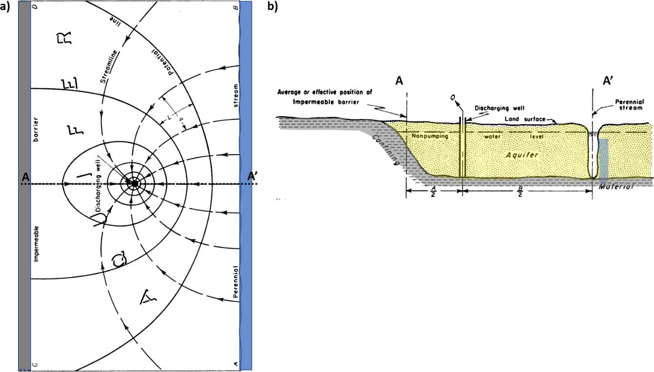
Figure Box 3‑1 ‑ Schematic showing a map view and a cross‑sectional view of an unconfined system bounded by a linear impermeable boundary and a parallel recharge boundary. a) A map view with groundwater flow lines and contours of water levels resulting from pumping a single well at a constant rate. Dashed arrows show groundwater flow and solid lines are water table elevation contours deceasing towards the well. b) Schematic cross section (A‑A’) of site conditions showing the location of a pumping well and the relation of the boundary conditions (modified from Ferris et al., 1962).
The setting depicted in Figure Box 3‑1 would seem to be straightforward as illustrated in the image well discussion in Section 11. However, the placement of initial image wells on each side of the two boundaries creates a more complex analysis. The image wells do not just interact with one boundary but affect both boundaries. For example, the pumping image well to the left of the impermeable boundary will affect the representation of the recharge boundary to the right. As one might guess, the presence of the injection image well to the right of the recharge boundary will also influence the impermeable boundary representation. Ferris and others (1962) explain that multiple appropriately spaced image wells are required to properly represent the final cone of depression for this two‑boundary setting. Ferris and others (1962) discuss this condition and other multiple‑boundary systems in their publication. Figure Box 3‑2a is from their publication and explains how the image wells were placed. This is illustrated in more detail in Figure Box 3‑2b. When an impermeable barrier is present, image wells representing the effect of the barrier must have the same sign for Q as the Q of the field well it reflects. When a recharge boundary is being represented by an image well it must have the opposite sign as Q for the field well. Thus, to represent a recharge boundary for a pumping well, the image well is an injection well which, mathematically, provides water that flows across the boundary. To represent a recharge boundary for an injection well, the image well is a pumping well which, mathematically, receives water that flows across the boundary representing the injected fluid flowing out to the feature that the boundary represented. This sounds complicated but is illustrated in Figure Box 3‑2. Ferris and others (1962) point out that, in theory, these combinations of image wells would extend to infinity. However, as the distance of the image wells from the boundaries increases the magnitude of their influence decreases and is less and less significant to the composite drawdown/drawup. For each image well the influence on the bounded water‑bearing unit and drawdown caused by the field well is additive, and the resulting cone of depression is a composite of all the calculated drawdowns within the cone.
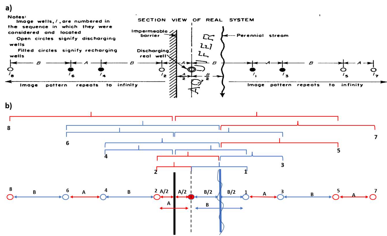
Figure Box 3‑2 ‑ Schematic of a map view of a pumping well bounded by both an extensive linear impermeable boundary and an extensive linear recharge boundary (Figure Box 3‑1). a) Ferris and others (1962) representation of the location and type of image wells needed to generate a composite data set to construct a cone of depression for a specified time. They note that for this geometry the pattern of image wells repeats from what is shown and theoretically extends to infinity. b) An interpretation of how the image wells were located. A and B are the spacing of the initial image wells from the boundaries. Blue arrows, brackets and open circles are representative of recharge (injection) image wells. Red arrows, brackets and red open circles are representative of impermeable boundary image wells (pumping). Image well 1 is an injection well that has a reverse sign on Q from the pumping well to represent the recharge boundary. Image well 2 is a pumping well that has the same sign as Q of the pumping well to represent the impermeable boundary. Image well 3 represents the reflection of image well 2 across the recharge boundary thus it has the opposite sign on Q as compared to image well 2. Image well 4 represents the reflection of image well 1 across the impermeable boundary thus it has the same sign on Q as compared to image well 1. Image well 5 represents the effect of the recharge boundary on image well 4 so it has opposite sign on Q as image well 4. Image well 6 represents the effect of the impermeable boundary on image well 5 so it has the same Q as image well 5. Image well 7 represents the reflection of image well 6 across the recharge boundary so it has the opposite sign. Image well 8 represents the reflection of image well 7 across the impermeable boundary so it has the same sign. The addition of image wells continues to infinity but soon they are far enough from the physical area between the impermeable and recharge boundaries that the additional drawdown is insignificant (modified from Ferris et al., 1962).