
Box 5 AQTESOLV
AQTESOLV V4.5 (aqtesolv.com) provides multiple methods to analyze hydraulic tests for confined, leaky confined, unconfined, and fractured aquifers as described in Figure 99 of Section 13.1 of this book. Automatic curve matching executes a nonlinear weighted least‑squares parameter estimation method that includes singular value decomposition. Statistical analyses of the fit between the data and the theoretical curve are provided (e.g., residual plots and standard error analysis).
When curve matching, the author recommends getting close to the parameter values by initially matching the field data with a Cooper‑Jacob straight‑line analysis. Once approximate values of T and S are generated, a more appropriate model that represents the actual aquifer conditions is selected. An example of automatic curve matching is presented in Figure Box 5‑1 showing both the type curve and derivative curve.
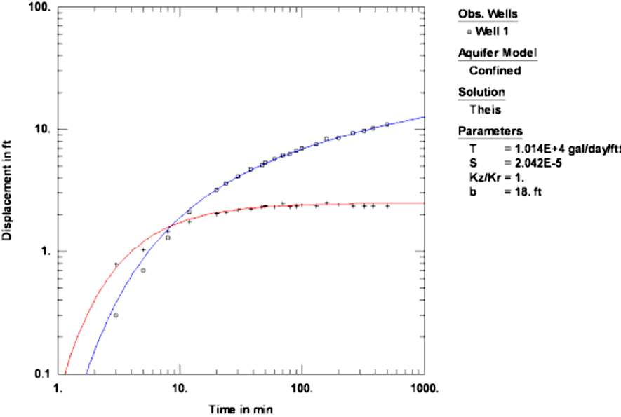
Figure Box 5‑1 ‑ Example of the match of a drawdown (displacement on the y axis) versus time curve (open squares) for observation well 1 with the Theis type curve (blue line). The derivative curve for the field data (plus signs) and type curve for the derivative (red curve) are also shown. T is in units of gallons/day/foot, the anisotropy ratio is 1 and the thickness of the pumped aquifer (b) is 18 ft (from the AQTESOLV V4.5 User’s Guide, 2004–2007; aqutesolve.com↗).
A second example of matching field data is illustrated for a leaky confined aquifer using the Hantush‑Jacob equation that considers water leakage to the confined unit by vertical flow through a confining bed from an overlying groundwater source (Figure Box 5‑2).
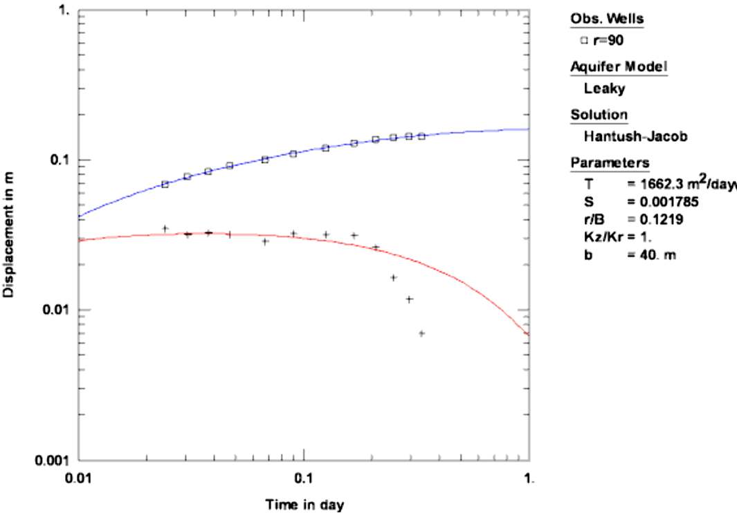
Figure Box 5‑2 ‑ Example of an automatic curve match of observation well data finished in a leaky confined aquifer to a theoretical Hantush‑Jacob curve. The blue line is the type curve match, and the red line is the time‑drawdown derivative match to the type curve derivative data. The Hantush‑Jacob model was used to determine T and S values. A second fit was attempted using the Hantush model, however, an analysis of the standard error suggested the Hantush model fit had greater uncertainty. Values of T in m2/d, S, and r/B are derived. r/B is r/(T/(K’b’)0.5 where K’ is the vertical hydraulic conductivity of the confining bed and b’ is the confining bed thickness. The pumped aquifer has an anisotropy ratio of 1 and the aquifer thickness (b) is 40 m (from the AQTESOLV V4.5 User’s Guide, 2004–2007; aqutesolv.com↗).
The AQTESOLV V4.5 User’s Guide (2004–2007) provides an additional source of information and examples. Videos produced to demonstrate how the program can be used are available on the internet and some are referenced on the 2023 website (aqutesolv.com↗). The software developer recommends going directly to the website for information on the capabilities and applications (aqutesolv.com↗).