
Solution Exercise 1
A 0.2 m diameter production well finished in a confined sand aquifer was pumped continuously at 300 L/minute for 10 hours. The water levels in the pumping well and two observation wells appeared to stabilize at about 6 hours as shown in this image.
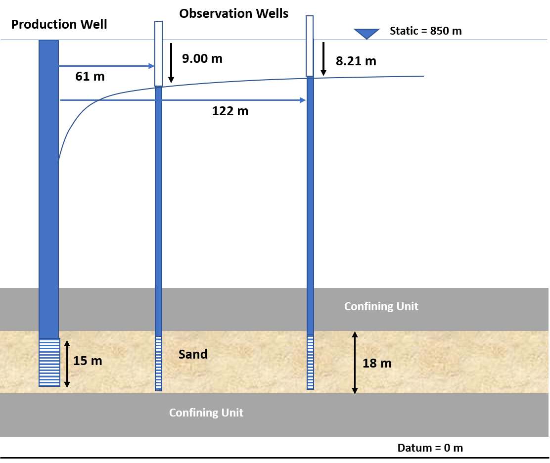
Cross section of a sand water bearing unit. The production well is pumped at a constant rate of 300 L/min for 10 hours and the drawdown in two observation wells is observed under what appear to be steady state conditions. Drawdowns from the static pre‑pumping water levels are shown along with the radial distances of wells from the production well.
- Assuming the pumping test reached steady state or pseudo steady state by 10 hours compute T and K.
The confined Thiem Equation (17) is applied to compute T under the stated conditions.
[latex]T = \frac{Q}{2\pi\left( h_{2} - h_{1} \right)}\ln\left( \frac{r_{2}}{r_{1}} \right)[/latex]
The values of h1 and h2 are equal to the static water level, 850 m, minus the reported steady state drawdown.
h1 = 850 m ‑ 9.00 m = 841.00 m
h2 = 850 m ‑ 8.21 m = 841.79 m
[latex]T = \frac{300\frac{L}{minute}\ \frac{{1\ m}^{3}}{1000\ L}\frac{1440\ minute}{d}}{2\ (3.14)\ (841.79\ m - 841.00\ m)}\ln\left( \frac{122\ m}{61\ m} \right) = 60\ \frac{m^{2}}{d}[/latex]
[latex]T = Kb\ \ so\ \ K = \frac{T}{b} = \frac{60\frac{m^{2}}{d}}{18\ m} = 3.4\ \frac{m}{d}[/latex]
- Do you need to account for the effects of partial penetration on the observation well data? Why or why not?
Pumping well partial penetration effects generally do not exceed a radial distance of 2b(Kh/Kv)0.5. Assuming the system is close to isotropic and homogeneous, then Kh/Kv = 1.
[latex]extent\ of\ partial\ penetration\ effects\ = \ 2b\left( \frac{K_{v}}{K_{h}} \right)^{0.5} = \ 2(18\ m)(1)^{0.5} = \ 36\ m[/latex]
Both observation wells are greater than 36 m from the pumping well, so partial penetration need not be accounted for.
- Assuming the production well radius is 0.1 m and the measured drawdown in the pumping well is 24 m, calculate the production well efficiency (i.e., measured drawdown divided by theoretical drawdown). A semi‑log plot of the observation well data will be helpful.
A semi log plot of drawdown versus distance is prepared using s=9.00 m at r=61 m and s=8.21 m at r=122 m and shown below.
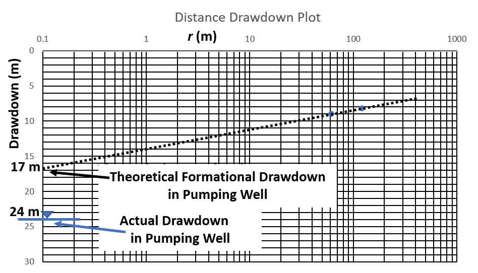
Drawdown at the two observation wells was plotted at the radial distance of each well. A straight line was fitted to the two data points (dashed black line). and extended back to the radius of the pumping well (0.1 m) where it is read from the graph as a theoretical drawdown of 17 m.
The well efficiency is computed as the theoretical drawdown (100 percent efficient) divided by the measured drawdown in the pumping well. Efficiency = 17 m / 24 m = 0.71 or 71 percent efficient.