
Solution Exercise 6
A discussion of interpreting single well pumping tests methods used to evaluate a well performance test is presented (Section 12). Though performance test data has limitations (e.g., uncertainty related to: the nature and location of water bearing units in the well, pumping water levels, and well loss during pumping), approximations of T can be made. Most commonly, performance test data are found on driller’s logs when a well is constructed. Review the well log presented in the image below.
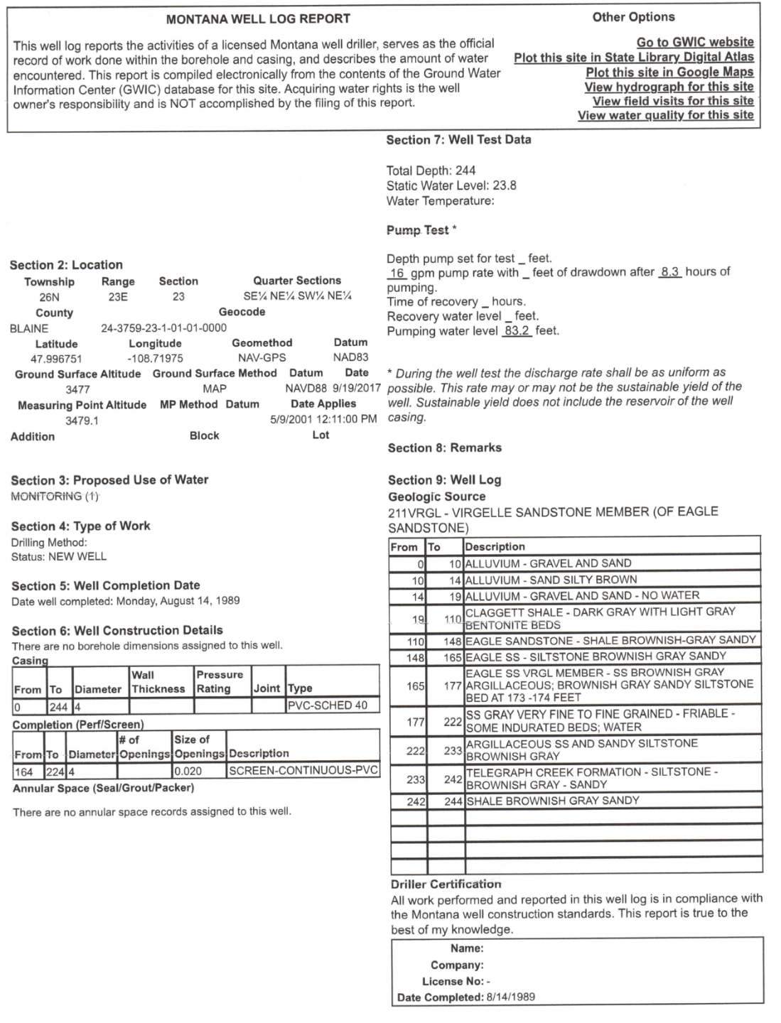
Example of a driller’s well log report for the completion of a well in Montana, USA. All length units are reported in feet and pumping rate is in gallons per minute. This log provides information on the static water level at the time of drilling, performance testing data including a pumping rate, length of the test, and the pumping level at the end of the test. It also shows a geologic log of the borehole. The owner of the well has been deleted from the figure.
Using this driller’s log answer the following questions:
- What depth interval and geologic material did the driller perforate to produce water to the well?
As shown in the image below, the perforated interval is screened with a continuous screen between 164 and 224 feet (50‑68 m). Geologically, this includes much of the Eagle Sandstone formation.
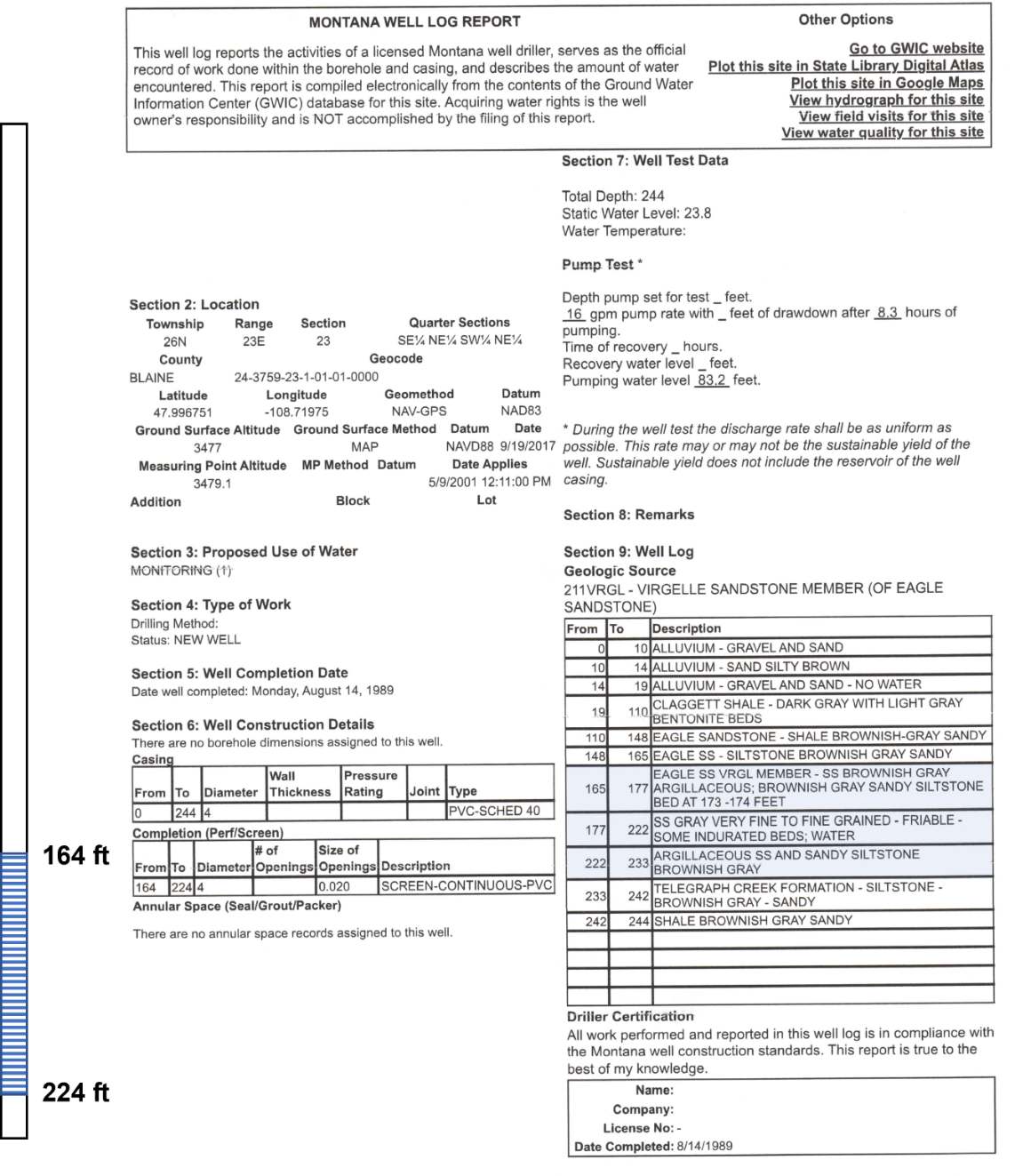
Well log showing the location of the screened interval and the corresponding geologic formations producing water (light blue shading). All units are in feet and discharge is in gallons per minute.
- Is this water producing unit likely confined or unconfined? Support your answer.
The water bearing zone is overlain by almost 100 feet (33 m) of shale and the static water level of the screened interval is above the top of the sandstone hydrogeologic unit (23.8 feet, 7.3 m). The presence of the confining shale and the position of the potentiometric surface supports that the water bearing unit is confined.
- Examine the static water level and performance test information, compute the specific capacity of the well.
The specific capacity is defined by Equation (99).
[latex]Specific\ Capacity = \ \frac{Q}{s_{F}}[/latex]
In this case, the pumping rate is 16 gallons per minute (60.5 L/min), and the drawdown is 83.2 feet ‑ 23.8 feet = 59.4 feet (18.1 m).
[latex]Specific\ Capacity = \ \frac{16\frac{gallons}{minute}}{59.4\ feet} = \ \frac{0.27\ gpm}{foot}[/latex]
[latex]Specific\ Capacity = \ \ \frac{60.5\frac{liters}{minute}\frac{1\ m^{3}}{1000\ liters}\frac{1440\ minute}{1\ d}}{18.1\ m} = \frac{4.8\frac{m^{3}}{d}}{m}[/latex]
- Based on the pumping data recorded by the driller, estimate the transmissivity of the aquifer using two methods. When applying each method justify your approach.
- Method 1: Assume the pumping has not proceeded to a steady state.
The Cooper‑Jacob approximation method presented in Equation (101) can be used to estimate T in terms of the specific capacity.
[latex]\frac{Q}{s} = \frac{1}{\frac{1}{4\pi T}\ 2.30\ log\left( 2.25\ \frac{Tt}{r_{w}^{2}S} \right)}[/latex]
Well specific data include, rw = 4 inches/2, and 2 in = 0.05 m, and t = 8.3 h = 0.125 d. The storativity is estimated for the sandstone (i.e., sound rock) based on concepts presented in Box 2 of Section 20 and using the data presented in Table Box 2‑2 (Ss=3.24×10‑6 m‑1).
[latex]S\ = \ S_{s}b[/latex]
The water bearing unit thickness, b, is assumed to be approximated by the screened interval, 224 feet – 164 feet = 60 feet (18.3 m).
[latex]S\ = \ \frac{0.00000324}{m}(18.3\ m) = 0.00006[/latex]
Then values of T are input and corresponding values of Q/s generated, then the results are plotted as a log‑log plot of T versus Q/s in the image following the calculations.
[latex]\frac{Q}{s} = \frac{1}{\frac{1}{4(3.14)10\frac{m^{2}}{d}}\ 2.30\ log\left\{ 2.25\ \frac{10\frac{m^{2}}{d}\ 0.125\ d}{(0.05m)^{2}(0.00006)} \right\}} = \frac{7.5\frac{m^{3}}{d}}{m}[/latex]
[latex]\frac{Q}{s} = \frac{1}{\frac{1}{4\ (3.14)\ 100\frac{m^{2}}{d}}\ 2.30\ log\left\{ 2.25\ \frac{100\frac{m^{2}}{d}\ 0.125\ d}{{(0.05\ m)}^{2}\ (0.00006)} \right\}} = \frac{66\frac{m^{3}}{d}}{m}[/latex]
[latex]\frac{Q}{s} = \frac{1}{\frac{1}{4\ (3.14)\ 1000\frac{m^{2}}{d}}\ 2.30\ log\left\{ 2.25\ \frac{1000\frac{m^{2}}{d}\ 0.125\ d}{{(0.05\ m)}^{2}\ (0.00006)} \right\}} = \frac{589\frac{m^{3}}{d}}{m}[/latex]
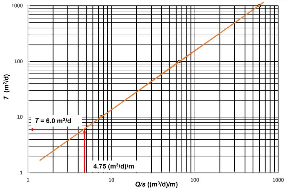
Log‑log plot of T versus Q/s for the well presented on the driller’s log. The Cooper‑Jacob method was used to calculate values of Q/s for T=10, 100, and 1,000 m2/d. The values were plotted. The orange line is a straight‑line fit to the data.
The specific capacity of the well is 4.75 (m3/d)/m and the value of T is read from the graph for that specific capacity as T = 6.0 m2/d.
- Method 2: Assume the pumping has resulted in near steady state conditions (simple equation approximation).
As discussed in Section 12 and presented by Equation (102), T for confined conditions can be estimated as follows.
[latex]T = 1.39\left( \frac{Q}{s} \right) = 1.39\left( \frac{4.8\frac{m^{3}}{d}}{m} \right) = 6.7\frac{m^{2}}{d}[/latex]
This equation assumes Q/s is a constant as it would be for steady state conditions. This value is close to the previous transient analyses, possibly because the pumping level was near steady state.
- When you only have performance data for a single pumping well do you anticipate the formational values of T will be greater or less than the values you computed? Why?
Generally, performance test data contain well loss and, depending on the well design, effects of partial penetration. One or both conditions would result in reported drawdown being greater than if the well was 100 percent efficient and fully penetrating (perforations greater than 80 to 85 percent of the unit thickness). This well would be considered fully penetrating. However, the effect of well loss is unknown. Thus, the drawdown likely includes well loss. Thus, an estimate of T is likely less than the formational T because Q/s would be smaller than if no well loss occurred.