
9.2 Hantush‑Jacob Solution (Leaky Confined‑No Water Released from Aquitard Storage)
Hantush and Jacob (1954) developed an equation that describes conditions in a leaky confined system without the effects of release of additional water from storage within a confining aquitard (Figure 41). The following subsections present the mathematical development of the Hantush‑Jacob equation and application of the method.
Formulation of the Hantush‑Jacob Equation
Equation (42) is the Hantush‑Jacob solution describing flow in leaky confined aquifer without the effects of release from aquitard storage.
| [latex]s(r,t) = \frac{Q}{4\pi T}\ \int_{\frac{r^{2}S}{4Tt}}^{\infty}{\ \frac{1}{y}\ exp\ \left\{ - y - \frac{r^{2}}{4B^{2}y}\ \right\}}\ dy[/latex] | (42) |
|---|
where:
| s(r,t) | = | drawdown at distance r, at time t (L) |
|---|---|---|
| Q | = | discharge (L3T‑1) |
| T | = | transmissivity (L2T‑1) |
| r | = | radial distance to an observation well (L) |
| S | = | storativity of the confined aquifer (dimensionless) |
| t | = | time (T) |
| r | = | radial distance (L) |
| u | = | r2S/(4Tt) |
| y | = | variable of integration (dimensionless) |
| B | = | (Tb’/K’)0.5 |
| b’ | = | saturated thickness of the confining unit (L) |
| K’ | = | vertical hydraulic conductivity of the confining unit (LT‑1) |
| r/B | = | r/(Tb’/K’)0.5 (dimensionless) |
The Hantush‑Jacob equation is written using the Hantush‑Jacob well function, W(u,r/B) as shown in Equation (43).
| [latex]s(r,t) = \frac{Q}{4\pi T}\ W\left( u,\frac{r}{B}\ \right)[/latex] | (43) |
|---|
where:
| s(r,t) | = | drawdown at a radial distance r at a time t (L) |
|---|---|---|
| Q | = | constant pumping rate (L3T‑1) |
| T | = | confined aquifer transmissivity (L2T‑1) |
| W(u,r/B) | = | Hantush‑Jacob well function (integral) (dimensionless) |
The well function incorporates two variables, u and r/B as shown in Equation (44).
| [latex]u = \frac{r^{2}S}{4Tt}\ \ \ \ ,\ \ \ \ \ \ \frac{r}{B} = \frac{r}{\sqrt{\frac{Tb'}{K'}}}[/latex] | (44) |
|---|
where:
| r | = | radial distance to an observation well (L) |
|---|---|---|
| S | = | storativity of the confined aquifer (dimensionless) |
| T | = | confined aquifer transmissivity (L2T‑1) |
| t | = | time since the pumping started (T) |
| B | = | (Tb’/K’)0.5 |
| K’ | = | vertical hydraulic conductivity of a confining unit (LT‑1) |
| b’ | = | thickness of confining bed (L) |
The vertical hydraulic conductivity of the confining unit (K’) divided by the confining unit thickness, b’, is referred to as vertical leakance (Anderson et al., 2015). Values for W(u,r/B) have been tabulated by Hantush (1956) and are presented in Figure 43.
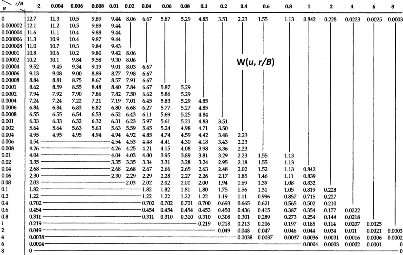
Figure 43 ‑ Table of selected W(u,r/B), u and r/B values (modified from Fetter (2001) and Hantush (1956)).
The relationship between u, r/B and W(u,r/B) is illustrated in Figure 43. As u and r/B become smaller, values of W(u,r/B) become larger. Figure 44 displays type curves created by plotting selected values of W(u,r/B) versus 1/u for different values of r/B. Figure 44 illustrates that as values of 1/u increase, values of W(u,r/B) for a given r/B begin to approach constants. The smaller the r/B value, the longer values of W(u,r/B) mirror the Theis type curve (W(u)). If r/B is very small, the leaky confined equation becomes the Theis equation where confining beds are assumed to be impermeable.
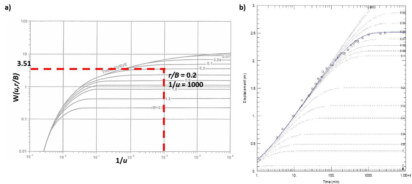
Figure 44 ‑ Hantush‑Jacob type curves for the leaky confined aquifer with vertical flow through the confining bed without the release of water from confining bed storage. a) The Theis curve is plotted for a reference (fully confined). The dashed red lines illustrate the relationship between 1/u, r/B and W(u,r/B). b) Generation of type curves for r/B = 0.01‑2.00. Y axis displacement is drawdown. Open circles and blue line are test data match to r/B = 0.06 (modified from Lohman (1972), Kasenow (2003), and AQTESOLV v4.5, www.aqtesolv.com↗.
The table of values (Figure 43) and the plotted type curves (Figure 44) represent a subset of values that are generated by substituting combinations of u and r/B into the analytical solution to produce values of W(u,r/B). If type curves with other values of r/B than shown in Figure 44 are required, they can be generated using the available analytical solution (e.g., Hantush & Jacob, 1954). When an analytical solution is not available, most often table or type curve data sets are linearly interpolated using data tables or figures like Figure 44.
Predicting Drawdown in Leaky Confined System with the Hantush‑Jacob Equation
The drawdown in a production well or observation wells at any radial distance at any time can be computed for the Hantush‑Jacob leaky confined setting. Solution inputs include a constant pumping rate (Q), the radial distance to the observation point (r), the confined unit transmissivity and storativity (T and S), and the vertical hydraulic conductivity and thickness (K’ and b’) of the aquitard. Again, the general simplifying assumptions are applicable (Section 6.3), such as the aquifer is isotropic and homogeneous, and flow in the confined aquifer is essentially horizontal. Values used in the equations must have compatible units so that drawdown is reported in length units.
Example
We forecast the drawdown at a distance of 17.9 m from a well pumping a constant rate of 500 L/min (720 m3/d) for 0.1 day in a 30 m thick sand and gravel aquifer. The confined aquifer has a transmissivity of 200 m2/d and a storativity of 0.0003. The confined aquifer is overlain by a sequence of aquitards and aquifers. The overlying aquitard is 40 m thick and has a vertical hydraulic conductivity of 1.0 m/d. The underlying confining unit is considered impermeable and has a very low hydraulic conductivity (on the order of 0.01 m/d). Using Equations (43) and (44) the value of r/B can be computed as follows.
[latex]\frac{r}{B} = \frac{17.9\ m}{\sqrt{\frac{200\ \frac{m^{2}}{d}40\ m}{1.0\ \frac{m}{d}}}} = 0.2[/latex]
Next u is computed as shown here.
[latex]u = \frac{({17.9m)}^{2}0.0003}{4\ \left( 200\ \frac{m^{2}}{d} \right)\ 0.1\ d} = 0.001[/latex]
Then, using Figure 43, the W(u,r/B) corresponding to these values is about 3.51. Now using Equation (43), drawdown is calculated at a distance of 17.9 m after 0.1 d of pumping at a constant rate of 720 m3/d as follows.
[latex]s(17.9\ m,\ 0.1\ d) = \frac{720\ \frac{m^{3}}{d}}{4\ (3.14)\ 200\ \frac{m^{2}}{d}}\ 3.51 = 1.0\ m[/latex]
The values presented in Figure 43 provide a limited data set. A plot of the table and additional values are provided as the Hantush‑Jacob type curves in Figure 44. These can also be used to obtain a value of W(u,r/B) when values of 1/u and r/B are known. For the example above when the point corresponding to 1/u = 1000 and r/B = 0.2 is plotted on the set of type curves in Figure 44, the well function is read from the y axis as W(u,r/B) = 3.51.
Pumping Test Data from a Confined Aquifer with a Leaky Confining Bed Without Additional Water Released from Aquitard Storage
Early‑time drawdown data from a pumping test in a leaky confined system will initially mirror the Theis curve, as nearly all water being pumped is initially derived from release of water from storage within the pumped unit. However, as leakage from adjacent lower hydraulic conductivity units begins to make up a portion of the pumping well discharge, the rate of drawdown will begin to decline such that the time‑drawdown data will no longer mirror the Theis type curve. If the total leakage rate through the confining layer becomes equal to the pump discharge rate, the drawdown in the leaky confined aquifer will cease declining and stabilize (plateau). An example of test data from a leaky confined aquifer with vertical flow through the confining bed is presented in Figure 45.
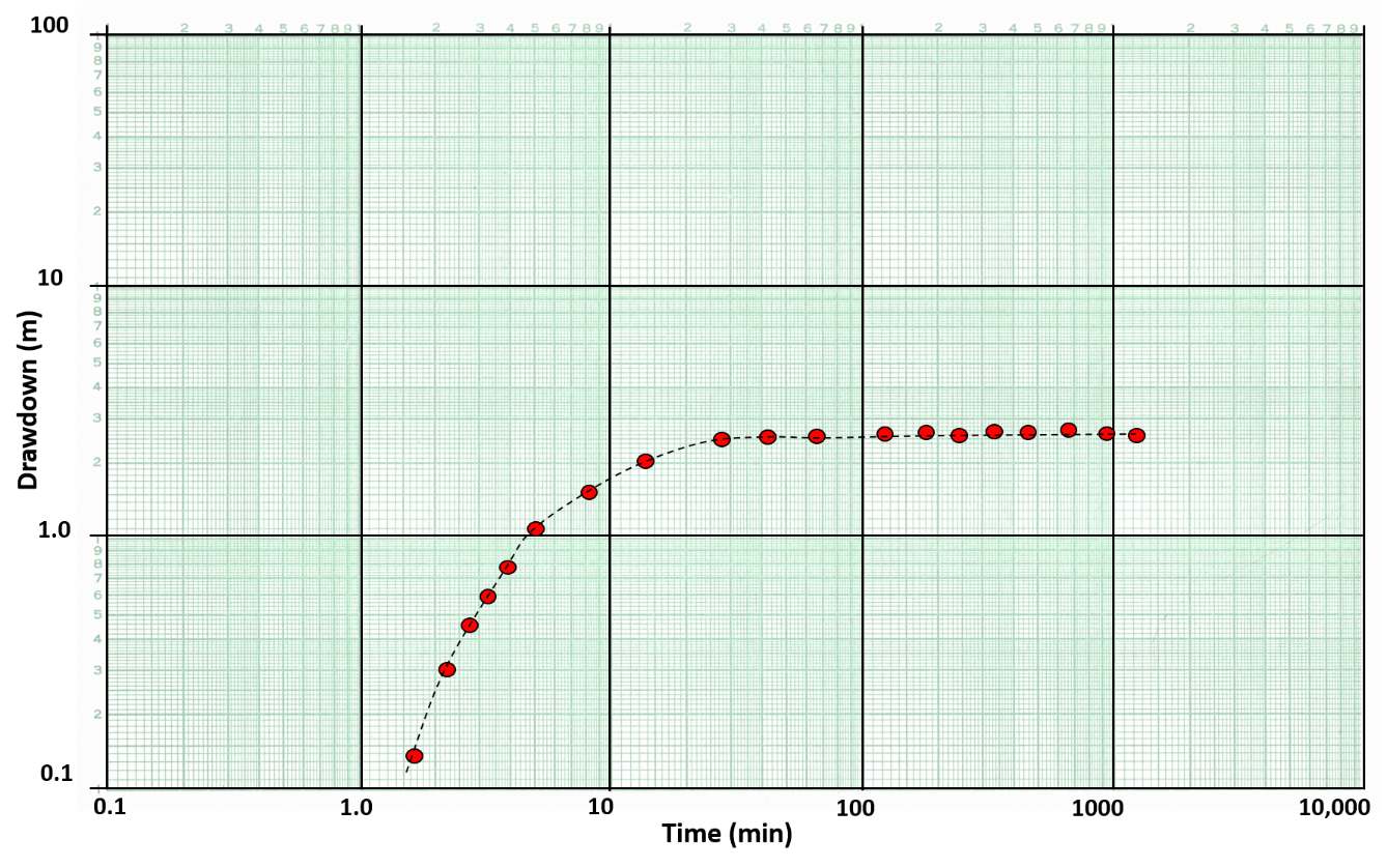
Figure 45 ‑ A schematic of time‑drawdown data for an observation well located 100 m from a well pumping at a constant rate of 2,500 m3/d for 1 day. The confined unit being pumped is a 50 m thick sand and gravel that is overlain by a 25 m thick confining unit. Data from the pumping test is plotted on log‑log scales. The red dots are measured drawdown and the dashed black line is hand fitted to the curve.
Hantush‑Jacob Curve Matching Method for a Pumping Test in a Confined Aquifer with a Leaky Confining Bed Without Water Released from Aquitard Storage
A process similar to the Theis curve matching method described in Section 8.3 is applied here. A set of leaky confined aquifer log‑log type curves are used (Figure 46). A plot of the drawdown and time data for an observation well is created using the same log‑log scale. While keeping the axes parallel, the field data are matched to a type curve as described for the Theis method previously (Figure 46).
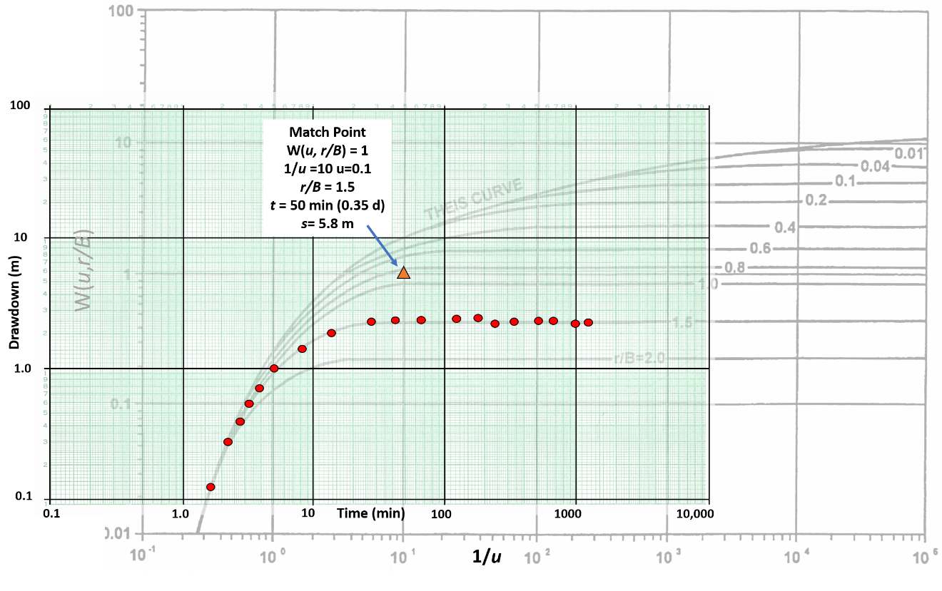
Figure 46 ‑ Curve match method for an aquifer test of a leaky confined aquifer with vertical flow in the confining bed. The data are shown in red dots and the match point is an orange triangle.
If values fall between plotted r/B values, a value is linearly interpolated between the two adjacent values or computed from the analytical solution. A match point is selected in the overlapping fields and values of r/B, 1/u, W(u,r/B), s, and t are determined.
Estimates of T and S for the leaky confined unit can be derived using the five match point values. T is computed using Equation (45) and the storativity, S, using Equation (46) (S). The vertical hydraulic conductivity, K’, of the aquitard is derived using Equation (46).
| [latex]T = \frac{Q}{4\pi s}\ W\left( u,\frac{r}{B} \right)[/latex] | (45) |
|---|
where:
| [latex]S = \frac{u4Tt}{r^{2}}\ \ \ \ \ \ ,\ \ \ \ \ K' = \frac{Tb'\left( \frac{r}{B} \right)^{2\ }}{r^{2}}[/latex] | (46) |
where:
| r | = | radial distance to observation point (L) |
|---|---|---|
| S | = | storativity of the confined aquifer (dimensionless) |
| T | = | confined aquifer transmissivity (L2T‑1) |
| t | = | time since the pumping started (T) |
| u | = | variable of integration derived from the curve match (dimensionless) |
| r/B | = | r/(Tb’/K’)0.5 |
| K’ | = | vertical hydraulic conductivity of confining bed (LT‑1) |
| b’ | = | thickness of confining bed (L) |
Example
The data for this example are listed in Figure 45. Assume drawdown is measured at an observation well located 100 m from a well pumping at a constant rate of 2,500 m3/d. The confined water‑bearing unit is overlain by a semi‑permeable aquitard that is 25 m thick and underlain by a low permeability confining unit. The match point values are listed on Figure 45. Calculate T, S, and K’.
[latex]T = \frac{2500\frac{m^{3}}{d}}{4\ (3.14)\ 5.8\ m}\ (1) = 34.3\frac{m^{2}}{d}[/latex]
[latex]S = \frac{(0.1)\ (4)\ 34.3\frac{m^{2}}{d}\ 0.35\ d}{{(100\ m)}^{2}} = 0.00048[/latex]
[latex]K' = \frac{34.3\frac{m^{2}}{d}\ 25\ m(1.5)^{2\ }}{{(100\ m)}^{2}} = 0.19\ \frac{m}{d}[/latex]
Hantush Inflection‑Point Method for a Pumping Test in a Confined Aquifer with a Leaky Confining Bed Without Water Released from Aquitard Storage
Hantush (1956) developed a method to determine the hydraulic properties of a leaky confined water‑bearing unit receiving water from vertical flow through the confining bed using a semi‑log plot of the time‑drawdown data from an observation well. If the thickness of the confining unit is known, the vertical hydraulic conductivity of the confining units can also be computed. Though this sounds like an easier approach, it involves additional mathematical tools. An example time‑drawdown plot for an observation well is presented in Figure 47.
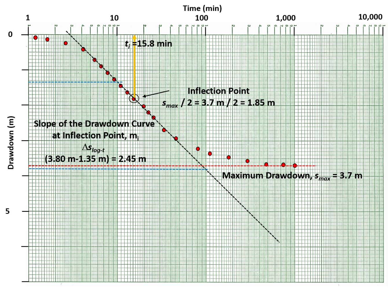
Figure 47 ‑ A schematic semi‑log plot of observation well data for a leaky confined formation. A straight‑line plot is created, and the maximum drawdown is identified. The inflection point (drawdown value) is defined as ½ the maximum drawdown. The time associated with the inflection point is noted as is the difference in drawdown over one log cycle of time, ∆slog‑t (defined by the blue dashed lines). Equations presented in this section are used to estimate T and S.
The Hantush (1956) inflection‑point method has several steps. Fetter (2001) summarized them as follows.
- Produce a semi‑log plot of time‑drawdown data for an observation well as shown in Figure 47. Select a value for the maximum drawdown. If the data has not stabilized (i.e., reached equilibrium), project the drawdown curve to estimate a maximum drawdown.
- The inflection point is defined as ½ of the maximum drawdown.
- Determine the time associated with the inflection point and the slope of the straight‑line portion of the curve over one log cycle of time. Hantush (1956) presents several useful relationships to define the inflection point as shown in Equations (47), (48), (49), (50), and (51).
| [latex]u_{i} = \frac{r^{2}S}{4Tt_{i}} = \frac{r}{2B}[/latex] | (47) | |
|---|---|---|
| [latex]m_{i} = \frac{2.3Q}{4\pi T}\exp\left( \frac{- r}{B} \right)[/latex] | (48) | |
| [latex]s_{i} = 0.5\ \left( s_{\max} \right) = \frac{Q}{4\pi T}K_{0\ }\left( \frac{r}{B} \right)[/latex] | (49) | |
| [latex]B = \left( \frac{T}{\frac{K'}{b'}} \right)^{0.5}[/latex] | (50) | |
| [latex]f\left( \frac{r}{B} \right) = \ \frac{2.3\ s_{i}}{m_{i}} = {\exp\left( \frac{r}{B}\ \right)}{K_{0}\left( \frac{r}{B}\ \right)\ }[/latex] | (51) |
where:
| ui | = | value of u at the inflection point (dimensionless) |
|---|---|---|
| r | = | radial distance from the pumping well to the observation well (L) |
| S | = | storativity of the confined aquifer (dimensionless) |
| T | = | transmissivity of the confined aquifer (L2T‑1) |
| ti | = | time at the inflection point mi (T) |
| B | = | defined in Equation (50) (L) |
| mi | = | slope of drawdown over one log cycle of time at the inflection point (dimensionless) |
| Q | = | constant discharge rate (L3T‑1) |
| si | = | drawdown at the inflection point (L) |
| smax | = | maximum drawdown (plateaued or projected to plateau) (L) |
| K0 | = | Bessel function zero‑order of the second kind (dimensionless) |
| K’ | = | vertical hydraulic conductivity of the confining unit (LT‑1) |
| b’ | = | thickness of the confining unit (L) |
| f(r/B) | = | function of r/B (dimensionless) |
As the values of si and mi can be derived as discussed earlier, and as shown on Figure 47, the value of f(r/b) is computed. With a value for f(r/b), r/b can be found by solving the second part of Equation (51). Function tables for f(x) = exp (x)K0(x) are shown in Figure 48.
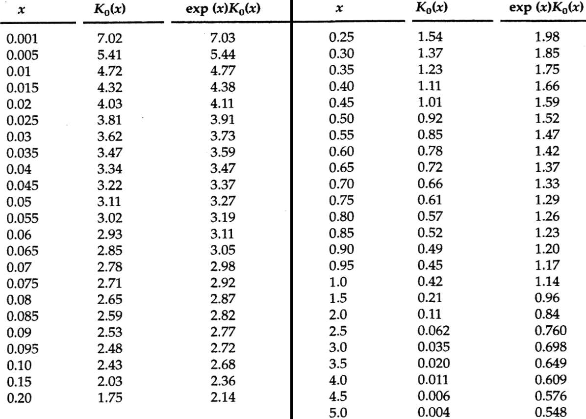
Figure 48 ‑ Values for f(x) = exp(x)K0(x) where x in the Hantush inflection method is equal to r/B (Hantush,1956).
The inflection method then derives hydraulic properties of the leaky confined aquifer using Equations (52) and (53).
| [latex]T = \frac{QK_{0}\left( \frac{r}{b} \right)}{2\pi s_{\max}}[/latex] | (52) | |
|---|---|---|
| [latex]S = \frac{4Tt_{i}}{2rB}[/latex] | (53) |
Example
The example shown in Figure 47 is used here to compute T and S for the leaky confined aquifer with vertical flow through the confining bed. Assume the observation well is located 75 m from the pumping well (Q = 4,250 m3/d) and the leaky confining unit is 15 m thick; then the following approach is used:
[latex]s_{\max} = \ 3.7\ m[/latex]
[latex]s_{i} = \ 1.8\ m[/latex]
[latex]t_{i} = \ 15.8\ min\ (0.011\ d)[/latex]
[latex]m_{i} = \ 2.45\ \frac{m}{\min}[/latex]
then
[latex]f\left( \frac{r}{B} \right) = \ \frac{2.3\ (1.8\ m)}{2.45\ \frac{m}{\min}} = \ 1.7[/latex]
Using the relationship f(r/B) = 1.7 = exp(r/B)K0(r/B), then from Figure 48, the value is between exp(x)K0(x) = 1.66 and exp(x)K0(x) = 1.75. The interpolation is shown below.
| x | K0(x) | exp (x) K0(x) |
|---|---|---|
| 0.40 | 1.11 | 1.66 |
| 0.37 (interpolated) | 1.16 (interpolated) | 1.7 |
| 0.35 | 1.23 | 1.75 |
Given that x = 0.37 m, with the observation well located 75 m from the pumping well, then B = 75 m / 0.37 = 203 m. Now using Equation (52).
[latex]T = \frac{4250\ \frac{m^{3}}{d}\ 1.16}{2\ (3.14)\ 3.7\ m} = 212\frac{m^{2}}{d}[/latex]
S is then computed from Equation (53).
[latex]S = \frac{4\ \left( 212\ \frac{m^{2}}{d} \right)\ 0.011d}{2\ (75\ m)\ (203\ m)} = 0.0003\ = \ 3x10^{- 4}[/latex]
Now since the thickness of the confining unit is known, 15 m, an estimate of the vertical hydraulic conductivity, K’, can be made using Equation (54).
| [latex]K' = \frac{Tb'}{B^{2}}[/latex] | (54) |
|---|
where:
| K’ | = | vertical hydraulic conductivity of the confining bed (LT‑1) |
|---|---|---|
| T | = | transmissivity of the confined aquifer (L2T‑1) |
| b’ | = | thickness of the confining unit (L) |
| B | = | defined in Equation (50) |
[latex]K' = \frac{212\frac{m^{2}}{d}\ 15\ m}{(203\ m)^{2}} = 0.08\frac{m}{d}[/latex]